Analysis

Assisted

Big picture

This dataset shows the spending, incentives, private investment, bill savings, and energy savings for all impacted middle income hh which received the assisted project incentives for WNY.

Explanation of variables: Overall spending: total cost of the project for all of WNY Overall incentives: the amount of money that the program gave to the project for all of WNY Overall private investment: equal to the difference between overall spending for all of WNY and overall incentive Overall bill savings: first year modeled energy bill savings for households in the program, versus their energy bill cost before the program for all of WNY Overall energy savings: estimated annual kwh savings in energy for all of WNY

In [1]:

# Load data_prep variables saved in previously run session
library(tidyverse)

── Attaching core tidyverse packages ──────────────────────── tidyverse 2.0.0 ──
✔ dplyr     1.1.4     ✔ readr     2.1.5
✔ forcats   1.0.0     ✔ stringr   1.5.1
✔ ggplot2   3.5.1     ✔ tibble    3.2.1
✔ lubridate 1.9.3     ✔ tidyr     1.3.1
✔ purrr     1.0.2     
── Conflicts ────────────────────────────────────────── tidyverse_conflicts() ──
✖ dplyr::filter() masks stats::filter()
✖ dplyr::lag()    masks stats::lag()
ℹ Use the conflicted package (<http://conflicted.r-lib.org/>) to force all conflicts to become errors

library(tigris)

To enable caching of data, set `options(tigris_use_cache = TRUE)`
in your R script or .Rprofile.

library(tidycensus)
library(janitor)


Attaching package: 'janitor'

The following objects are masked from 'package:stats':

    chisq.test, fisher.test

library(sf)

Linking to GEOS 3.11.1, GDAL 3.6.2, PROJ 9.1.1; sf_use_s2() is TRUE

options(tigris_use_cache = TRUE)
library(scales)


Attaching package: 'scales'

The following object is masked from 'package:purrr':

    discard

The following object is masked from 'package:readr':

    col_factor

library(RColorBrewer)

load("/workspaces/reports/data/temp/energy_efficiency_push_buffalo/data_prep_env.RData")

# Define colors
sky <- "#68bed8"
midnight_lighter <- "#0b6082"

In [2]:

county_projectstats_assisted_wny <- county_projectstats_assisted_wny |>
  mutate(total_private_investment = total_project_cost - total_incentives)

region_projectstats_assisted_wny <- county_projectstats_assisted_wny |>
  summarize_if(is.numeric, sum, na.rm=TRUE)

Underlying assumptions to be added: 1. We are assuming that one project is equal to one household. This is because we do not have direct HH information from the assisted dataset but since it is residential projects we have inferred that each project is a hh.

How much money was spent overall in WNY (via assisted incentives)? Answer: $ 18,081,182

How much private investment did that catalyze? Answer: $ 41,853,095

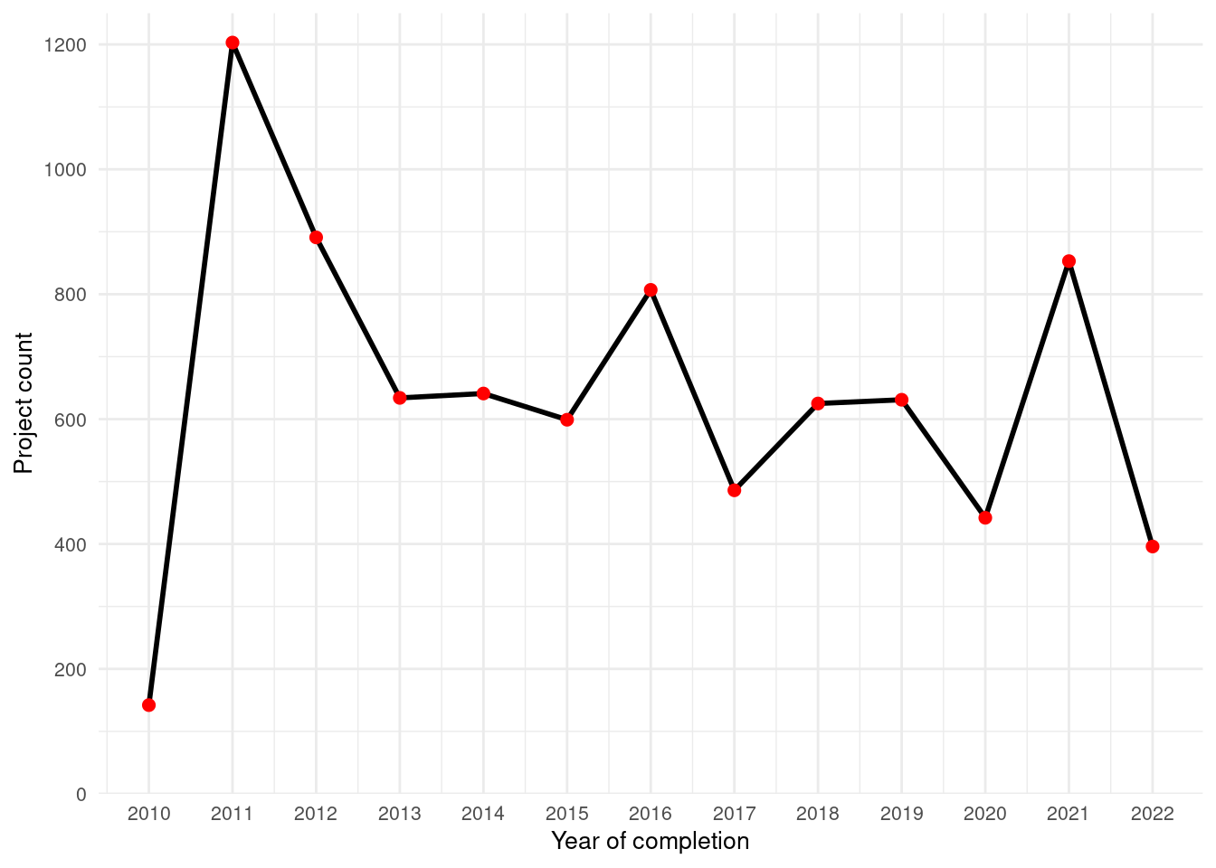
How many projects were completed over time?

Answer: Overall, 8,401 Assisted projects were completed in this time period.

See timeseries graph below

In [3]:

# Comments say last 2 years should be excluded but code includes 2022?
region_projectcountbyyear_assisted_wny <- projects_assisted |>
  filter(county %in% wny_counties) |> 
  mutate(completion_year = year(project_completion_date)
  ) |>
1  filter(!completion_year %in% c(2023)) |>
  summarise(
    project_count_by_year = n(),
    .by = completion_year
  )

1: The last two years are excluded because there have been fewer projects completed during this time (some might still be in process or started later).

2011: 1203 projects completed 2022: 396 projects completed

In [4]:

ggplot(region_projectcountbyyear_assisted_wny, 
        aes(x = completion_year,
            y = project_count_by_year, 
            group = 1)) +
        geom_line(color = "black", linewidth = 1) +
        geom_point(color = "red", size = 2) +
        labs(
            x = "Year of completion",
            y = "Project count",
        ) +
        scale_y_continuous(breaks = seq(0, 1200, 200), limit = c(0, 1250), expand = c(0, NA)) +
        scale_x_continuous(
          breaks = unique(region_projectcountbyyear_assisted_wny$completion_year), 
          labels = unique(region_projectcountbyyear_assisted_wny$completion_year)
        ) +
        theme_minimal() +
        theme(
          plot.title = element_text(size = 14, face = "bold"),
          axis.title = element_text(size = 10),
          axis.text = element_text(size = 8),
          plot.caption = element_text(size = 8, hjust = 1)
      )

Number of completed Assisted projects by year

It seems like there was a drop of projects completed in 2017 and 2020 - could the drop in 2020 be because of the pandemic?

What was spent by county in terms of incentives and what private investment was generated?

Allegany
- Allegany county spent: 166,236
- Allegany county had private investment of: 432,662
Cattaraugus:
- Cattaraugus county spent: 181,951
- Cattaraugus county had private investment of: 569,183
Chautauqua:
- Chautauqua county spent: 485,055
- Chautauqua county had private investment of: 1,539,345
Erie:
- Erie county spent: 14,212,326
- Erie county had private investment of: 32,223,251
Niagara:
- Niagara county spent: 3,035,614
- Niagara county had private investment of: 7,088,654

Graph showing incentives and private investment by county in WNY:

In [5]:

county_projectstats_assisted_wny_long <- 
  county_projectstats_assisted_wny |>
  select(county, total_incentives, total_private_investment) |>
  pivot_longer(
    cols = c(total_incentives, total_private_investment),
    names_to = "category",
    values_to = "value"
  ) |>
  mutate(
    category = factor(
      category, 
      levels = c("total_private_investment", "total_incentives")
    )
  )

The overwhelming majority of incentive and out-of-pocket spending in WNY went to Erie county, followed by Niagara.

In [6]:

# Spending category ratio
county_spendingratio_assisted_wny <- county_projectstats_assisted_wny |>
  mutate(total_spending_pct = total_project_cost / sum(total_project_cost),
  investment_incentive_ratio = total_private_investment / total_incentives)

In [7]:

In [8]:

county_spendingratio_assisted_wny |>
  select(c(county, investment_incentive_ratio)) |>
  mutate(investment_incentive_ratio = paste0(format(round(investment_incentive_ratio, 2), nsmall = 2), "-to-1")) |>
  knitr::kable(col.names = c("County",
                           "Spending ratio"))

Assisted program: Out-of-pocket spending to incentives ratio by county

County	Spending ratio
Erie	2.27-to-1
Niagara	2.34-to-1
Allegany	2.60-to-1
Cattaraugus	3.13-to-1
Chautauqua	3.17-to-1

In [9]:

# Spending by beneficiary
county_projectstats_assisted_wny <- county_projectstats_assisted_wny |>
  mutate(spending_by_beneficiary = total_project_cost / total_projects,
  incentives_by_beneficiary = total_incentives / total_projects,
  private_investment_by_beneficiary = total_private_investment / total_projects)

In [10]:

county_projectstats_assisted_wny_long |>
  ggplot(aes(x = county, y = value, fill = category)) +
  geom_bar(stat = "identity") +
  geom_text(
    aes(label = paste0("$", scales::comma(value/1000000, accuracy = 0.1), "M")), 
    position = position_stack(vjust = 0.5), 
    color = "white", 
    size = 3.5
  ) +
  scale_fill_manual(
    values = c(
      "total_incentives" = sky, 
      "total_private_investment" = midnight_lighter
    ),
    labels = c(
      "total_incentives" = "Incentives", 
      "total_private_investment" = "Out-of-pocket Spending"
    )
  ) +
  scale_y_continuous(labels = scales::comma) + 
  labs(
    x = "County",
    y = "Spending amount (USD)",
    fill = "Category"
  ) +
  theme_minimal()

Incentives and Out-of-pocket Spending by County

Graph showing bill savings per county in WNY:

In [11]:

county_projectstats_assisted_wny |>
ggplot(aes(x = county, y = total_bill_savings)) +
  geom_bar(stat = "identity", fill = "skyblue") +
  geom_text(aes(label = scales::comma(total_bill_savings)), 
            vjust = -0.5, 
            color = "black", 
            size = 3.5) +
  scale_y_continuous(labels = scales::comma) + 
  labs(title = "Total first-year bill savings, by WNY county",
       x = "County",
       y = "Bill Savings (USD)") +
  theme_minimal()

Graph showing energy savings per county in WNY:

In [12]:

county_projectstats_assisted_wny |>
ggplot(aes(x = county, y = total_energy_savings)) +
  geom_bar(stat = "identity", fill = "skyblue") +
  geom_text(aes(label = scales::comma(total_energy_savings)), 
            vjust = -0.5, 
            color = "black", 
            size = 3.5) +
  scale_y_continuous(labels = scales::comma) + 
  labs(title = "Overall Energy Savings by County",
       x = "County",
       y = "Energy Savings (kWh)") +
  theme_minimal()

As expected, the charts for total first-year bill savings and total first-year energy savings mirror the chart for total spending.

Assisted is design to help moderate income households, between 60-80% AMI.

What percent of the potential beneficiaries in WNY were served by the program since 2010? (2 terms: eligible HHs, beneficiary HHs)

Answer: 12.1 percent #Minh, the code for this question is new <- to be double checked. it is the 2 cell blocks below.

In [13]:

# Percentage of HHs that received program assistance by region
region_mihh_wny <- zcta_hhlmi_wny |> 
  summarise(
    mi_households = sum(mi_households, na.rm = TRUE)
  )

region_totalstats_assisted_wny <- region_projectstats_assisted_wny |> 
  cross_join(region_mihh_wny) |> 
  mutate(beneficiary_hh_pct = (total_projects / mi_households) * 100  
)

In [14]:

# Percentage of HHs that received program assistance by county
county_mihh_wny <- zcta_hhlmi_wny |> 
  summarise(
    mi_households = sum(mi_households, na.rm = TRUE),
    .by = county
  )

county_totalstats_assisted_wny <- county_mihh_wny |> 
  inner_join(county_projectstats_assisted_wny, 
    by = join_by(county), 
    relationship = "one-to-one",
    unmatched = "error"
  )

county_totalstats_assisted_wny <- county_totalstats_assisted_wny |> 
  mutate(
    beneficiary_hh_pct = total_projects / mi_households
  )

In [15]:

In [16]:

county_totalstats_assisted_wny |>
  select(c(county, total_projects, total_project_cost, total_incentives, total_private_investment, total_bill_savings, total_energy_savings)) |>
  mutate(across(where(is.numeric), scales::label_comma())) |>
  mutate(across(c("total_project_cost", "total_incentives", "total_bill_savings", "total_private_investment"), function(x) paste0("$", as.character(x)))) |>
  knitr::kable(col.names = c("County",
                           "Projects count",
                           "Total project spending",
                           "Total incentives",
                           "Total out-of-pocket spending",
                           "Total bill savings",
                           "Total energy savings (kW)"))

Assisted program statistics by county

County	Projects count	Total project spending	Total incentives	Total out-of-pocket spending	Total bill savings	Total energy savings (kW)
Erie	6,534	$46,435,577	$14,212,326	$32,223,251	$2,304,157	2,036,992
Niagara	1,487	$10,124,268	$3,035,614	$7,088,654	$625,764	561,205
Cattaraugus	82	$751,134	$181,951	$569,183	$67,431	60,817
Chautauqua	236	$2,024,400	$485,055	$1,539,345	$122,442	244,897
Allegany	62	$598,898	$166,236	$432,662	$29,062	50,503

In [17]:

In [18]:

county_totalstats_assisted_wny |>
  select(c(county, mi_households, beneficiary_hh_pct)) |>
  mutate(across(c("beneficiary_hh_pct"), scales::label_percent(accuracy = 1))) |>
  mutate(across(where(is.numeric), scales::label_comma())) |>
  knitr::kable(col.names = c("County",
                           "MIHHs count",
                           "Beneficiary household percentage"))

Assisted program subsidy recipients

County	MIHHs count	Beneficiary household percentage
Erie	46,535	14%
Niagara	10,819	14%
Cattaraugus	3,626	2%
Chautauqua	6,160	4%
Allegany	2,154	3%

In [19]:

In [20]:

county_totalstats_assisted_wny |>
  select(c(county, spending_by_beneficiary, incentives_by_beneficiary, private_investment_by_beneficiary)) |>
  mutate(across(where(is.numeric), scales::label_comma())) |>
  mutate(across(c("spending_by_beneficiary", "incentives_by_beneficiary", "private_investment_by_beneficiary"), function(x) paste0("$", as.character(x)))) |>
  knitr::kable(col.names = c("County",
                           "Total spending",
                           "Incentives",
                           "Out-of-pocket spending"))

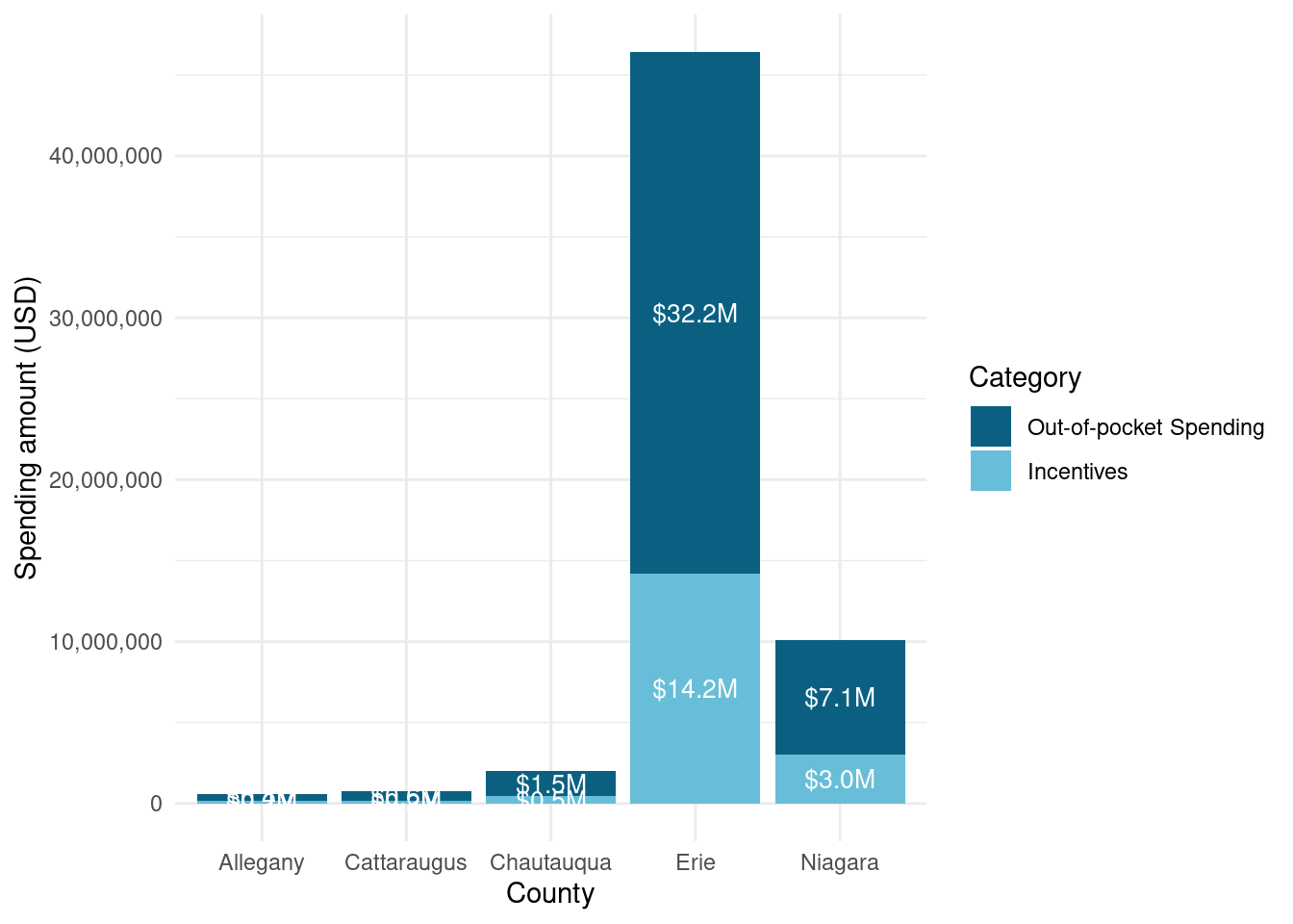
Assisted program measures per beneficiary household by county

County	Total spending	Incentives	Out-of-pocket spending
Erie	$7,107	$2,175	$4,932
Niagara	$6,809	$2,041	$4,767
Cattaraugus	$9,160	$2,219	$6,941
Chautauqua	$8,578	$2,055	$6,523
Allegany	$9,660	$2,681	$6,978

Percent of beneficiaries that benefitted by county:

Allegany: 2.8782 %
Cattaraugus: 2.2615 %
Chautauqua: 3.8309 %
Erie: 14.0412%
Niagara: 13.745 %

Assisted appears to have reached a 4-5x larger share of the eligible population in Erie and Niagara counties than in the others. Therefore, the outsized spending on these counties does not solely reflect higher population density.

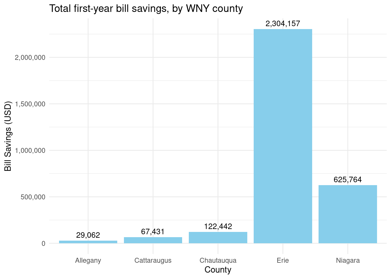
How many bill savings? Overall: 3,148,856
By county? - Allegany: 29,062 - Cattaraugus: 67,431 - Chautauqua: 122,442 - Erie: 2,304,157 - Niagara: 625,764

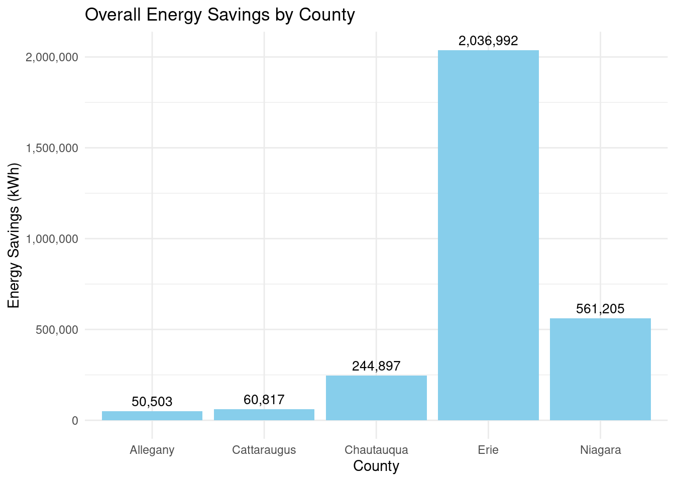
How many energy savings? Overall: 2,954,414 By county? - Allegany: 50,503 - Cattaraugus: 60,817 - Chautauqua: 24,4897 - Erie: 2,036,992 - Niagara: 561,205

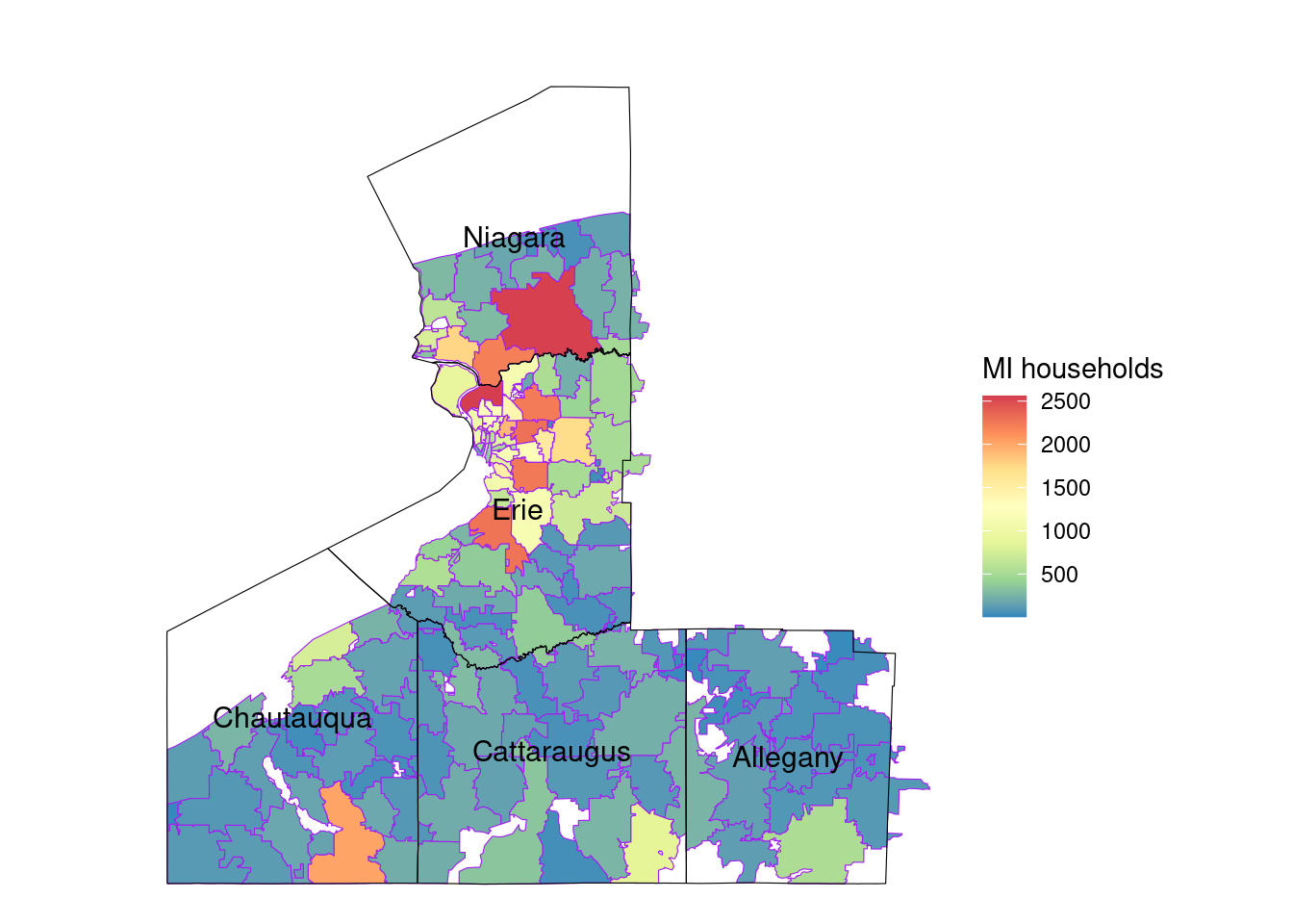
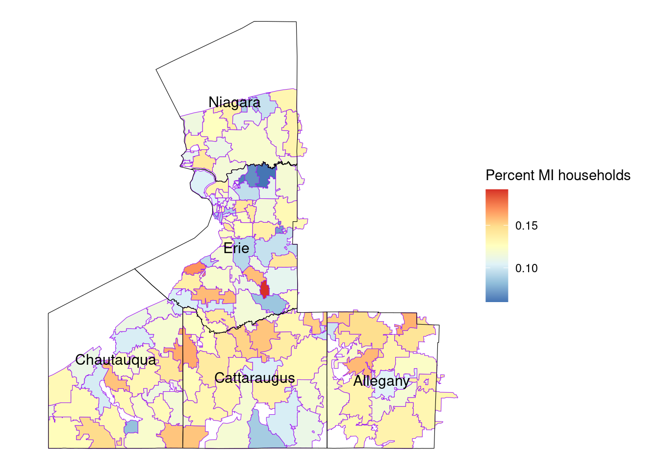
Geography

The data frame zcta_hhmi_assisted_wny -> zcta_totalstats_assisted_wny is created to show both hh level income information and project level information. It is on the zcta level.

In [21]:

zcta_hhmi_wny <- zcta_hhlmi_wny |> 
  select(-c(li_households, lmi_households, pct_li, pct_lmi)) 

zcta_totalstats_assisted_wny <- zcta_hhmi_wny |> 
  right_join(zip_projectstats_assisted_wny, 
    by = join_by(zcta == zip), 
1    relationship = "one-to-one",
  ) |> 
  filter(county != "NA")

1: In this right join, every zip in zip_projectstats_assisted_wny should find a zcta match in zcta_hhlmi_wny. Our final df should have 139 rows as in zip_projectstats_assisted_wny, which it does so we can proceed.

The df zcta_totalstats_bybeneficiary_assisted_wny is created to get total spending/saving numbers and to get spending/savings by assisted beneficiary.

In [22]:

zcta_totalstats_bybeneficiary_assisted_wny <- zcta_totalstats_assisted_wny |> 
  mutate(
    incentives_per_beneficiary_hh = total_incentives / total_projects, 
    billsavings_per_beneficiary_hh = total_bill_savings / total_projects, 
    energysavings_per_beneficiary_hh = total_energy_savings / total_projects,
    .keep = "used"
  )

Where are the potential beneficiaries?

To answer this question, we need to get geometry information:

In [23]:

zctas_ny_data <- zctas(state = "NY", year = 2010)

counties_ny_data <- counties(state = "NY", year = 2010)

zcta_boundary_wny <- zctas_ny_data |> 
  filter(ZCTA5CE10 %in% wny_zipcodes_list)

county_boundary_wny <- counties_ny_data |> 
  filter(NAME10 %in% wny_counties)

We are doing the join here to add the geometry information to the zcta_totalstats_assisted_wny df.

In [24]:

zcta_totalstats_assisted_wny_geom <- zcta_totalstats_assisted_wny |>
1  left_join(zcta_boundary_wny,
    by = join_by(zcta == ZCTA5CE10), 
    relationship = "one-to-one",
  )

1: It is expected that not all rows of zcta_boundary_wny will find a match, because there are some PO boxes/some ZCTAs that are not in the assisted project data. As long as our final df has the same number of zctas as zcta_totalstats_assisted_wny, we are fine - which it does.

We are making this a spatial data frame so that we can use ggplot to make the maps.

In [25]:

zcta_totalstats_assisted_wny_sf <- st_as_sf(zcta_totalstats_assisted_wny_geom)

Maps start here: showing all mi hh #TODO: hard to read map with polarizing heat color. Change palette #TODO: do we want a year here in the title?

In [26]:

zcta_totalstats_assisted_wny_sf |>
  ggplot() +
    geom_sf(aes(fill = mi_households), color = "purple") +
    geom_sf(data = county_boundary_wny, fill = NA, color = "black", size = 5) +  
    geom_sf_text(data = county_boundary_wny, 
                aes(label = NAME10), 
                size = 4, 
                color = "black") +  
    scale_fill_distiller(palette = "Spectral", 
                          name = "MI households", 
                          direction = -1) +
    theme_void() +
    labs(title = "",
  )

Warning in st_point_on_surface.sfc(sf::st_zm(x)): st_point_on_surface may not
give correct results for longitude/latitude data

Number of moderate income households, by zip code

Normalized map: mihh / totalhh #TODO: change color palette for clarity

In [27]:

zcta_totalstats_assisted_wny_sf |>
  ggplot() +
    geom_sf(aes(fill = mi_households / total_households), color = "purple") +
    geom_sf(data = county_boundary_wny, fill = NA, color = "black", size = 1) +  
    geom_sf_text(data = county_boundary_wny, 
                aes(label = NAME10), 
                size = 4, 
                color = "black") +  
    scale_fill_distiller(palette = "RdYlBu", 
                          name = "Percent MI households", 
                          direction = -1,
                        ) +
    theme_void()

Warning in st_point_on_surface.sfc(sf::st_zm(x)): st_point_on_surface may not
give correct results for longitude/latitude data

Percent of eligible households for Assisted program

Most counties seem to have fairly similar concentrations of eligible households (moderate income) with Allegany potentially being the highest.

#TODO: comment on geographical distribution/MI concentration

Data analysis for geography related questions at the county starts here:

In [28]:

county_beneficiaries_assisted_wny <- county_totalstats_assisted_wny |> 
  mutate(  
    potential_beneficiaries = mi_households,
    incentives_pct = (total_incentives / sum(total_incentives)) * 100,
    incentives_by_beneficiary = total_incentives / total_projects, 
    billsavings_by_beneficiary = total_bill_savings / total_projects, 
    energysavings_by_beneficiary = total_energy_savings / total_projects,
    .keep = "unused"
  ) |>
  select(-c(total_project_cost, beneficiary_hh_pct))

Where did this money go? By county:

Erie 78.6%
Niagara 16.8%
Chautauqua 2.68%
Cattaraugus 1.01%
Allegany 0.919%

Incentives over beneficiaries? By county:

Allegany 2681.
Cattaraugus 2219.
Chautauqua 2055.
Erie 2175.
Niagara 2041.

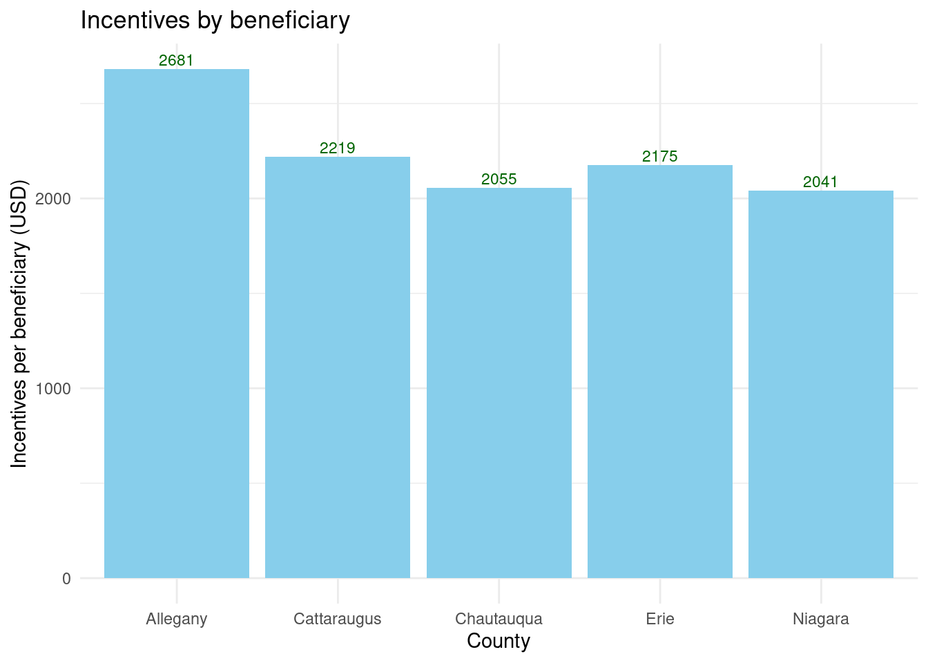
Allegany had the highest incentive dollar amount per beneficiary, while other counties were fairly similar in terms of amount.

Graph showing spending by beneficiary per county:

In [29]:

county_beneficiaries_assisted_wny |>
  ggplot(aes(x = county, y = incentives_by_beneficiary)) +
  geom_bar(stat = "identity", fill = "skyblue") +
  geom_text(
    aes(label = round(incentives_by_beneficiary)), 
    vjust = -0.3, 
    color = "darkgreen", 
    size = 3
  ) +
  labs(
    title = "Incentives by beneficiary", 
    x = "County", 
    y = "Incentives per beneficiary (USD)"
  ) +
  theme_minimal()

The average Assisted incentive was pretty comparable across counties, $2K and $2.2K. Allegany had a higher average, $2681, but this is largely an artifact of the very few projects that have take place there, less than 1% of the spending.

Bill savings over beneficiaries?

By county: - Erie 353. - Niagara 421. - Allegany 469. - Chautauqua 519. - Cattaraugus 822.

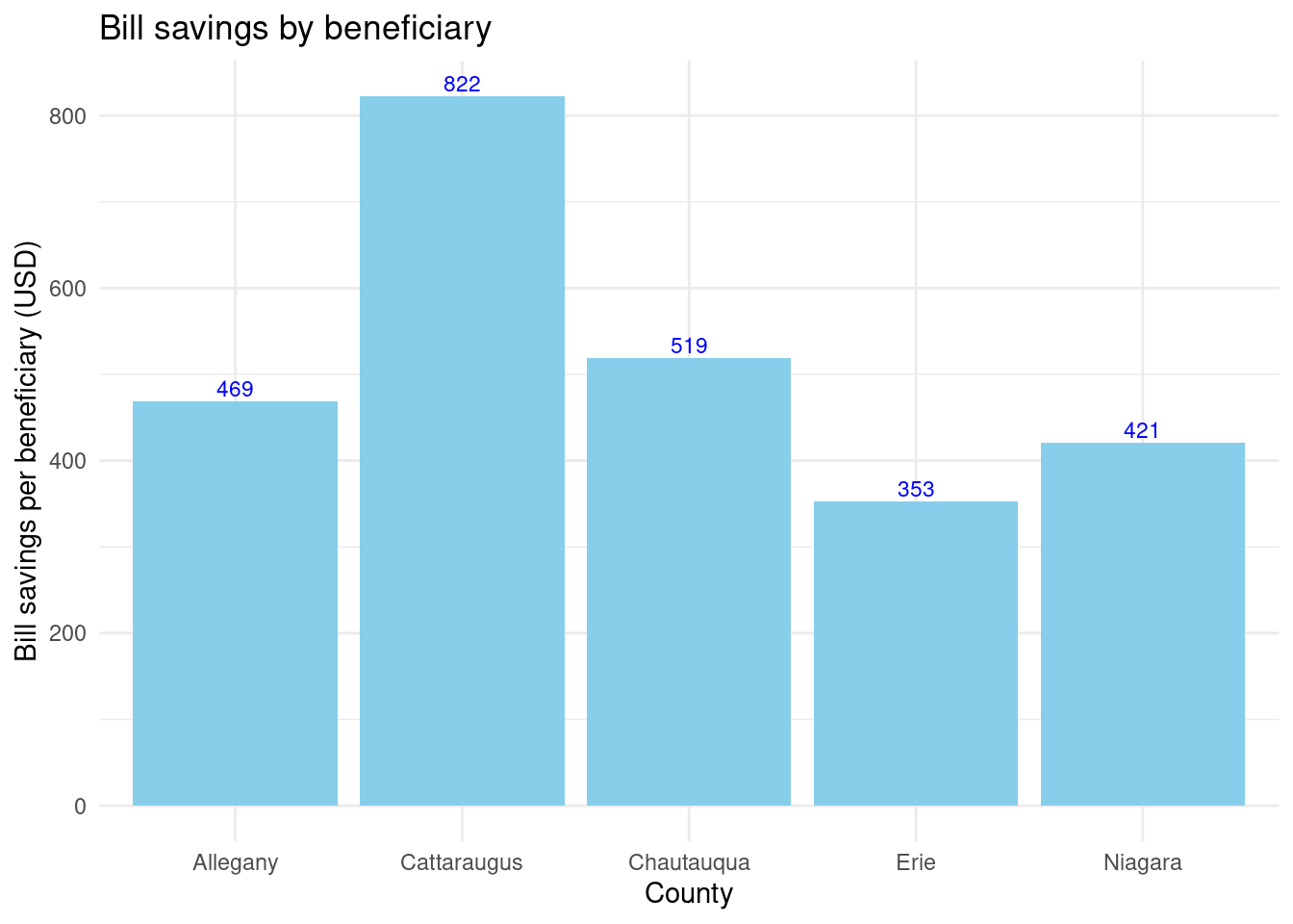
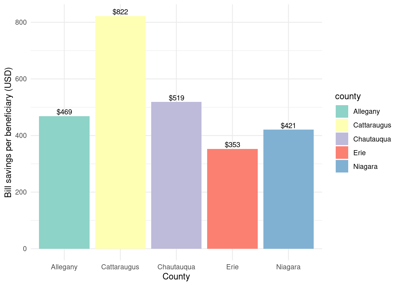
Graph showing bill savings by beneficiary per county:

In [30]:

county_beneficiaries_assisted_wny |>
  ggplot(aes(x = county, y = billsavings_by_beneficiary)) +
  geom_bar(stat = "identity", fill = "skyblue") +
  geom_text(
    aes(label = round(billsavings_by_beneficiary)), 
    vjust = -0.3, 
    color = "blue", 
    size = 3
  ) +
  labs(
    title = "Bill savings by beneficiary", 
    x = "County", 
    y = "Bill savings per beneficiary (USD)"
  ) +
  theme_minimal()

There’s more variation in first-year bill savings… rural counties seem to have higher savings on average.

According to the National Agricultural and Rural Development Policy Center (NARDeP), “residential per household energy consumption in rural areas is about 10% higher compard to urban areas.” Could be worth seeing if that is what is happening here?

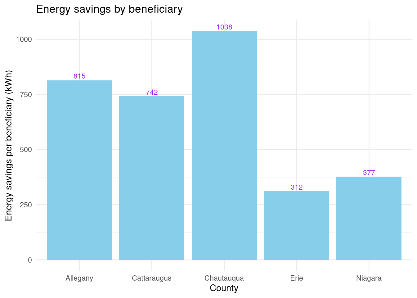
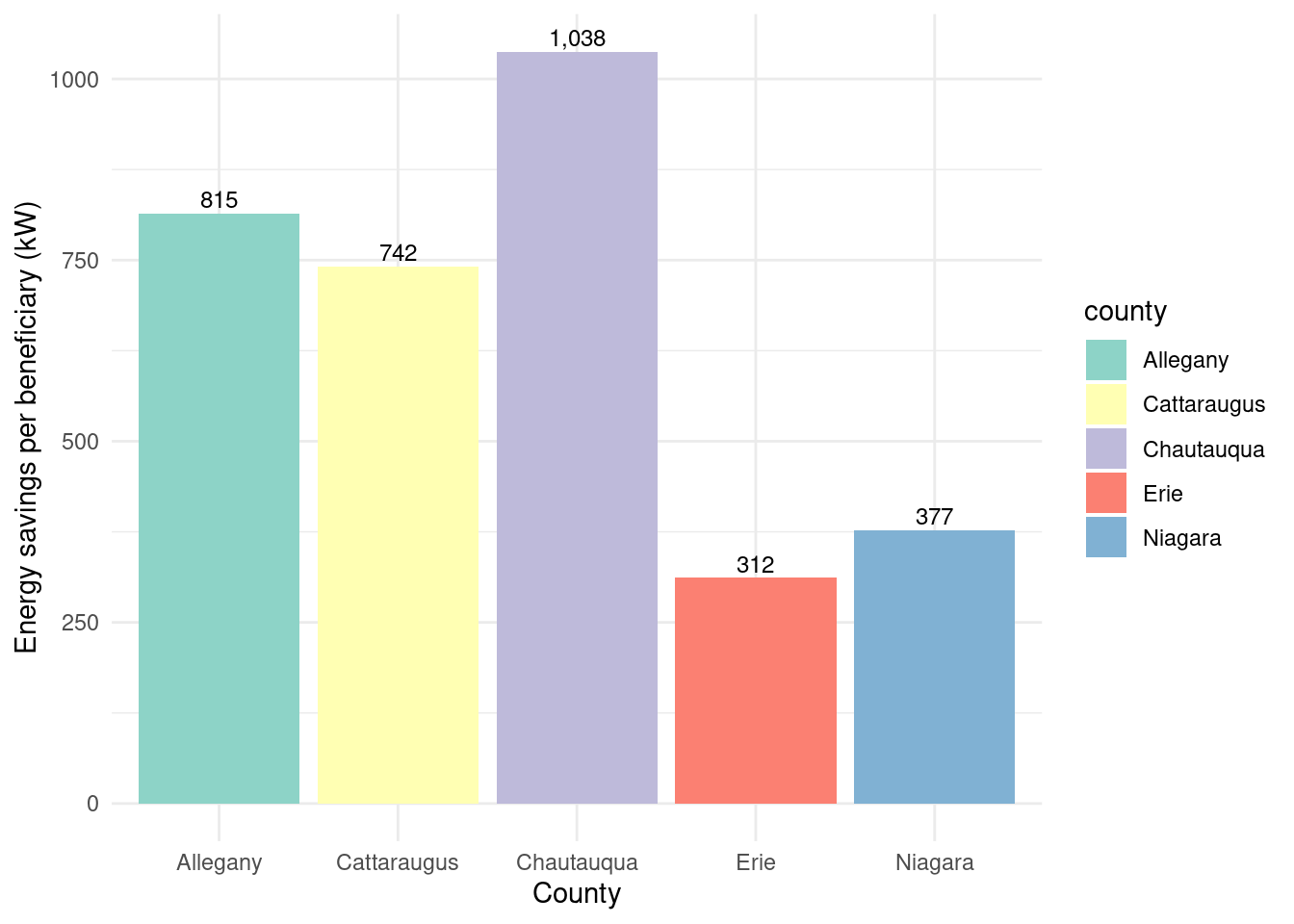
Source: https://aese.psu.edu/nardep/publications/policy-briefs/rural-energy-use-and-the-challenges-for-energy-conservation-and-efficiency#:~:text[…]f%202.69

Energy savings over beneficiaries? By county: - Erie 312. - Niagara 377. - Cattaraugus 742. - Allegany 815. - Chautauqua 1038.

Graph showing energy savings by beneficiary per county:

In [31]:

county_beneficiaries_assisted_wny |>
  ggplot(aes(x = county, y = energysavings_by_beneficiary)) +
    geom_bar(stat = "identity", fill = "skyblue") +
    geom_text(aes(label = round(energysavings_by_beneficiary)), vjust = -0.3, 
                  color = "purple", size = 3) +
    labs(title = "Energy savings by beneficiary", 
         x = "County", 
         y = "Energy savings per beneficiary (kWh)") +
    theme_minimal()

Erie and Niagara have the lowest energy and bill savings, but the correlation is less clear for the rural counties.

Unclear correlation by the numbers: - Cattaraugus has by far the highest bill savings by beneficiary with 822 but has considerably lower energy savings by beneficiary (742) than Chautauqua and Allegany. - Meanwhile Chautauqua and Allegany have lower bill savings/beneficiary with 519 and 469 respectivly but they have the highest energy savings by beneficiary with 1038 and 815 respectivly.

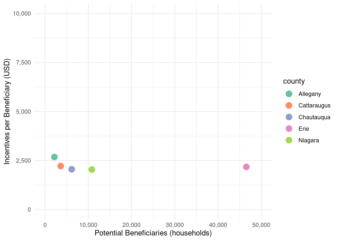
Does the average incentive amount vary depending on the size of the eligible population?

In [32]:

county_beneficiaries_assisted_wny |> 
  ggplot(aes(x = potential_beneficiaries, 
            y = incentives_by_beneficiary, 
            color = county)) +
  geom_point(size = 4) +
  labs(x = "Potential Beneficiaries (households)",
       y = "Incentives per Beneficiary (USD)") +
  theme_minimal() +
  scale_color_brewer(palette = "Set2") +
  scale_y_continuous(limits = c(0, 10000), labels = scales::comma) +
  scale_x_continuous(limits = c(0, 50000), labels = 
  scales::comma)

Assisted Incentives by Beneficiary vs. Potential Beneficiaries

Not really.

One potential question for further analysis would be variation in project size by county.

Multiple bar graph showing incentives + savings per county:

first pivoting the df + adding levels for order!

In [33]:

county_beneficiaries_assisted_wny_long <- county_beneficiaries_assisted_wny |>
  pivot_longer(
    cols = c(
      incentives_by_beneficiary, 
      billsavings_by_beneficiary, 
      energysavings_by_beneficiary
    ),
    names_to = "category",
    values_to = "value"
  ) |>
  mutate(category = factor(category, 
                           levels = c("incentives_by_beneficiary", 
                                      "billsavings_by_beneficiary", 
                                      "energysavings_by_beneficiary")))

In [34]:

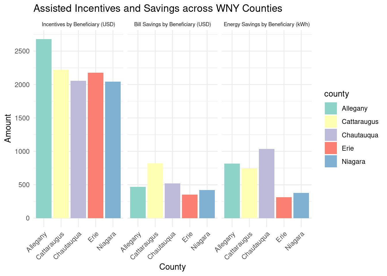
labels_for_graph <- as_labeller(c(
  "incentives_by_beneficiary" = "Incentives by Beneficiary (USD)",
  "billsavings_by_beneficiary" = "Bill Savings by Beneficiary (USD)",
  "energysavings_by_beneficiary" = "Energy Savings by Beneficiary (kWh)"
))

In [35]:

ggplot(county_beneficiaries_assisted_wny_long,
  aes(x = county, y = value, fill = county)) +
  geom_bar(stat = "identity") +
  facet_wrap(~category, scales = "fixed", labeller = labels_for_graph) +
  labs(title = "Assisted Incentives and Savings across WNY Counties",
       x = "County",
       y = "Amount") +
  theme_minimal() +
  scale_fill_brewer(palette = "Set3") + 
  theme(axis.text.x = element_text(angle = 45, hjust = 1), 
  strip.text.x = element_text(size = 7)) +
  scale_y_continuous(breaks = seq(0, 3000, 500))

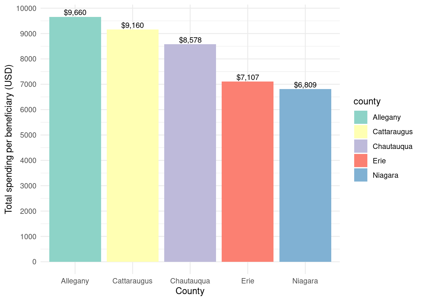
In [36]:

county_beneficiaries_assisted_wny |>
  ggplot(aes(x = county, y = spending_by_beneficiary, fill = county)) +
  geom_bar(stat = "identity") +
  theme_minimal() +
  labs(x = "County",
      y = "Total spending per beneficiary (USD)") +
  geom_text(aes(label = paste0("$", scales::comma(spending_by_beneficiary, accuracy = 1))),
          vjust = -0.3,
          color = "black",
          position = position_dodge(width = 0.9),
          size = 3.2) +
  scale_fill_brewer(palette = "Set3") +
  scale_y_continuous(breaks = seq(0, 10000, 1000))

Total project spending per beneficiary by county for Assisted program

In [37]:

county_beneficiaries_assisted_wny |>
  ggplot(aes(x = county, y = billsavings_by_beneficiary, fill = county)) +
  geom_bar(stat = "identity") +
  theme_minimal() +
  labs(x = "County",
      y = "Bill savings per beneficiary (USD)") +
  geom_text(aes(label = paste0("$", scales::comma(billsavings_by_beneficiary, accuracy = 1))),
          vjust = -0.3,
          color = "black",
          position = position_dodge(width = 0.9),
          size = 3.2) +
  scale_fill_brewer(palette = "Set3")

Bill savings per beneficiary by county for Assisted program

In [38]:

county_beneficiaries_assisted_wny |>
  ggplot(aes(x = county, y = energysavings_by_beneficiary, fill = county)) +
  geom_bar(stat = "identity") +
  theme_minimal() +
  labs(x = "County",
      y = "Energy savings per beneficiary (kW)") +
  geom_text(aes(label = scales::comma(energysavings_by_beneficiary, accuracy = 1)),
          vjust = -0.3,
          color = "black",
          position = position_dodge(width = 0.9),
          size = 3.2) +
  scale_fill_brewer(palette = "Set3")

Energy savings per beneficiary by county for Assisted program

Race

The df zcta_totalstats_assisted_wny also shows race information:

In [39]:

zcta_mihh_byrace_wny <- zctarace_hhlmi_wny |> 
  mutate(
    total_mihh = sum(mi_households, na.rm = TRUE), # total_mihh by zcta
    .by = c(zcta, county)
  ) |>
  rename(mihh_by_race = mi_households) |>
  select(-c(li_households, 
            lmi_households, 
            total_households, 
            pct_li, pct_mi,   
            pct_lmi)
  )

zcta_totalstats_assisted_wny <- zip_projectstats_assisted_wny |> 
1  left_join(zcta_mihh_byrace_wny,
    by = join_by(zip == zcta)
  ) |> 
2  filter(county != "NA")

zcta_totalstats_assisted_wny <- zcta_totalstats_assisted_wny |>
  mutate(
    mi_zcta_percent = mihh_by_race / total_mihh,
    assisted_spending_race = mi_zcta_percent * sum_project_cost,
    assisted_incentives_race = mi_zcta_percent * total_incentives,
    assisted_private_investment_race = 
      assisted_spending_race - assisted_incentives_race,
    assisted_billsavings_race = mi_zcta_percent * total_bill_savings,
    assisted_energysavings_race = mi_zcta_percent * total_energy_savings,
    assisted_totalprojects_race = mi_zcta_percent * total_projects,
    .by = c(zip,county)
  )

1: We use a left join here because we need to prioritize the zips in zip_projectstats_assisted_wny since those are the zips with projects in them. The resulting df should be 139 * 5 since there are 5 races (695 total), and it is, so we can move on.
2: The counties that are NA were removed because they did not find a match in dataset that was filtered for just midde income households.

We then get totals for the zcta_totalstats_assisted_wny and bring it down to the county level to create: county_totalstats_byrace_assisted_wny.

In [40]:

county_totalstats_byrace_assisted_wny <- zcta_totalstats_assisted_wny |> 
  summarize(
    assisted_spending_race = sum(assisted_spending_race, 
      na.rm = TRUE),
    assisted_incentives_race = sum(assisted_incentives_race, 
      na.rm = TRUE),
    assisted_privateinvestment_race = sum(assisted_private_investment_race,
      na.rm = TRUE),
    assisted_billsavings_race = sum(assisted_billsavings_race, 
      na.rm = TRUE),
    assisted_energysavings_race = sum(assisted_energysavings_race, 
      na.rm = TRUE),
    assisted_totalprojects_race = sum(assisted_totalprojects_race,
      na.rm = TRUE),
    assisted_mihh_race = sum(mihh_by_race, na.rm = TRUE),
    .by = c(county, race)
  )

The df region_incentives_byrace_assisted_wny is then created to get incentives by household by race for the entire region WNY.

In [41]:

region_incentives_byrace_assisted_wny <- 
  county_totalstats_byrace_assisted_wny |>
    summarize(
      total_incentives = sum(assisted_incentives_race),
      total_mihh = sum(assisted_mihh_race),
      .by = race) |>
    mutate(
      incentives_per_hh = total_incentives / total_mihh
  )

Graph showing race spending (Overall WNY)

In [42]:

region_incentives_byrace_assisted_wny |>
  ggplot(aes(x = race, y = incentives_per_hh, fill = race)) +
  geom_text(aes(label = paste0("$", scales::comma(incentives_per_hh, accuracy = 1))),
            vjust = -0.3,
            color = "black",
            position = position_dodge(width = 0.9),
            size = 3.2) +
  geom_bar(stat = "identity") +
  labs(x = "Race",
       y = "Incentives per Potential Beneficiary Household (USD)") +
  theme_minimal() +
  scale_fill_brewer(palette = "Set3")

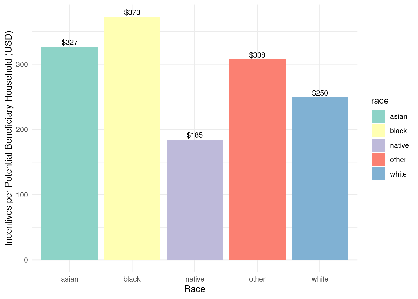
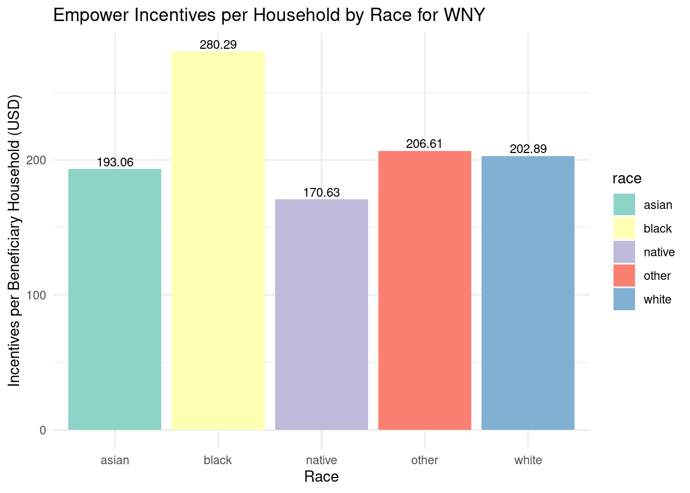
Assisted program incentives per household by race for WNY

Black households appear to have received the highest dollar amount of incentive per household, while Native American households received the least. Based on our analysis, this implies that more racially diverse ZCTAs received more funding.

county_totalstats_assisted_wny is also used to get a df that shows percent spending/savings

In [43]:

county_pctstats_byrace_assisted_wny <- 
  county_totalstats_byrace_assisted_wny |>
  mutate(
    spending_total = sum(
      assisted_spending_race, 
      na.rm = TRUE
    ), 
    incentives_total = sum(
      assisted_incentives_race, 
      na.rm = TRUE
    ),
    privateinvestment_total = sum(
      assisted_privateinvestment_race, 
      na.rm = TRUE
    ),
    billsavings_total = sum(
      assisted_billsavings_race,
      na.rm = TRUE
    ),
    energysavings_total = sum(
      assisted_energysavings_race, 
      na.rm = TRUE
    ), 
    totalprojects_total = sum(
      assisted_totalprojects_race, 
      na.rm = TRUE
    ),
    .by = county
  ) |> 
  mutate(
    spending_byrace_pct = 
      (assisted_spending_race / spending_total) * 100,
    incentives_byrace_pct = 
      (assisted_incentives_race / incentives_total) * 100,
    privateinvestment_byrace_pct = 
      (assisted_privateinvestment_race / 
      privateinvestment_total) * 100,
    billsavings_byrace_pct = 
      (assisted_billsavings_race / billsavings_total) 
      * 100,
    energysavings_byrace_pct = 
      (assisted_energysavings_race / energysavings_total) 
      * 100,
    totalprojects_byrace_pct = 
      (assisted_totalprojects_race / 
      totalprojects_total) * 100,
    .keep = "unused"
    ) |>
    select(-c(assisted_mihh_race) # irrelevant variable
  )

The same process is repeated but for all of WNY as opposed to by county:

In [44]:

region_totalstats_byrace_assisted_wny <- zcta_totalstats_assisted_wny |> 
  summarize(
    spending_total = sum(assisted_spending_race, 
      na.rm = TRUE),
    incentives_total = sum(assisted_incentives_race, 
      na.rm = TRUE),
    privateinvestment_total = sum(assisted_private_investment_race,
      na.rm = TRUE),
    billsavings_total = sum(assisted_billsavings_race, 
      na.rm = TRUE),
    energysavings_total = sum(assisted_energysavings_race, 
      na.rm = TRUE),
    totalprojects_total = sum(assisted_totalprojects_race,
      na.rm = TRUE),
    .by = c(race)
  )

In [45]:

region_pctstats_byrace_assisted_wny <-
 region_totalstats_byrace_assisted_wny |>
  mutate(
    spending_byrace_pct = spending_total / 
      sum(spending_total) * 100,
    incentives_byrace_pct = incentives_total / 
      sum(incentives_total) * 100,
    privateinvestment_byrace_pct = privateinvestment_total / 
      sum(privateinvestment_total) * 100,
    billsavings_byrace_pct = billsavings_total /
      sum(billsavings_total) * 100,
    energysavings_byrace_pct = energysavings_total /
      sum(energysavings_total) * 100,
    totalprojects_byrace_pct = totalprojects_total /
      sum(totalprojects_total) * 100,
    .keep = "unused"
  )

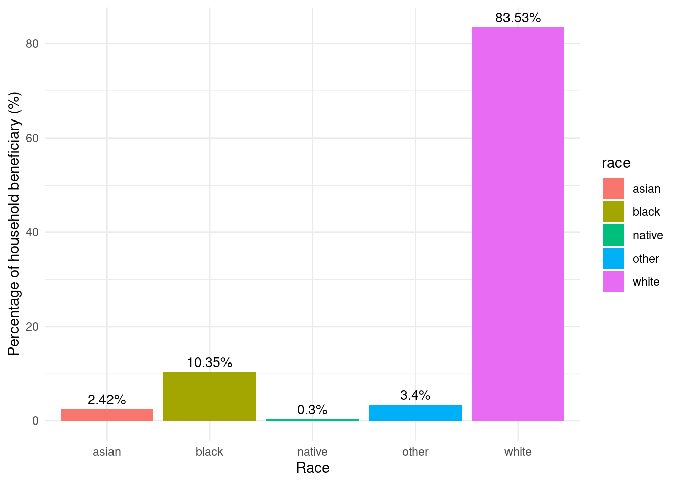
What percent of beneficiaries are white vs. black vs. native vs. other?

white 83.5%
black 10.4%
other 3.4%
asian 2.42%
native 0.301%

What percent of incentives went to white vs. black vs. native vs. other?

white 81.0
black 12.3
other 3.86
asian 2.51
native 0.318

What percent of energy savings went to white vs. black vs. native vs. other?

white 85.2
black 9.11
other 3.18
asian 2.24
native 0.304

By county, from county_pctstats_byrace_assisted_wny:

What percent of incentives went to white vs. black vs. native vs. other? - Allegany white 97.5
- Allegany black 0.101 - Allegany native 0.0802 - Allegany asian 0.283 - Allegany other 2.05
- Cattaraugus white 94.3
- Cattaraugus black 1.04
- Cattaraugus native 1.30
- Cattaraugus asian 0.792 - Cattaraugus other 2.59
- Chautauqua white 94.6
- Chautauqua black 0.695 - Chautauqua native 0.445 - Chautauqua asian 0.557 - Chautauqua other 3.72
- Erie white 77.7
- Erie black 14.7
- Erie native 0.216 - Erie asian 3.00
- Erie other 4.37
- Niagara white 92.8
- Niagara black 4.16
- Niagara native 0.732 - Niagara asian 0.692 - Niagara other 1.67

What percent of bill savings went to white vs. black vs. native vs. other?

1 Allegany white 97.6
2 Allegany black 0.112 3 Allegany native 0.0700 4 Allegany asian 0.261 5 Allegany other 1.93
6 Cattaraugus white 94.7
7 Cattaraugus black 0.632 8 Cattaraugus native 1.67
9 Cattaraugus asian 0.653 10 Cattaraugus other 2.36
11 Chautauqua white 95.0
12 Chautauqua black 0.718 13 Chautauqua native 0.339 14 Chautauqua asian 0.604 15 Chautauqua other 3.39
16 Erie white 80.3
17 Erie black 12.7
18 Erie native 0.193 19 Erie asian 2.87
20 Erie other 3.98
21 Niagara white 92.9
22 Niagara black 3.93
23 Niagara native 0.740 24 Niagara asian 0.739 25 Niagara other 1.68

What percent of energy savings went to white vs. black vs. native vs. other? 1 Allegany white 98.5
2 Allegany black -0.0236 3 Allegany native -0.0427 4 Allegany asian 0.117 5 Allegany other 1.49
6 Cattaraugus white 98.2
7 Cattaraugus black 0.155 8 Cattaraugus native -0.819 9 Cattaraugus asian 1.49
10 Cattaraugus other 0.965 11 Chautauqua white 94.8
12 Chautauqua black 0.638 13 Chautauqua native 0.339 14 Chautauqua asian 1.37
15 Chautauqua other 2.90
16 Erie white 81.1
17 Erie black 12.1
18 Erie native 0.198 19 Erie asian 2.84
20 Erie other 3.78
21 Niagara white 93.2
22 Niagara black 3.71
23 Niagara native 0.820 24 Niagara asian 0.716 25 Niagara other 1.53

In [46]:

# Incentives per HH by race by county
county_spending_byrace_assisted_wny <- 
  county_totalstats_byrace_assisted_wny |>
    rename(
      total_incentives = assisted_incentives_race,
      total_potential_beneficiaries = assisted_mihh_race,
    ) |>
    mutate(
      spending_per_potential_beneficiary = total_incentives / total_potential_beneficiaries,
    ) |>
    select(c(county, race, total_incentives, total_potential_beneficiaries, spending_per_potential_beneficiary))

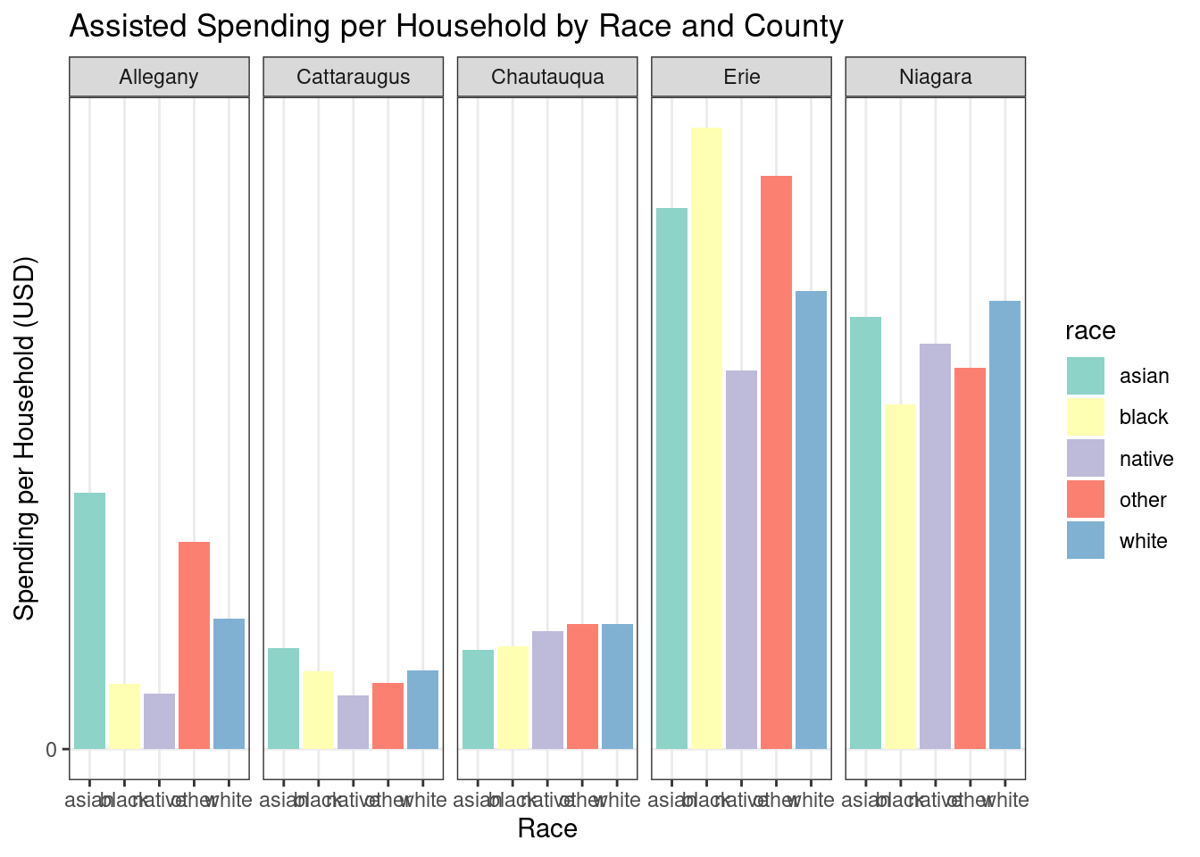
Graph showing race spending (By county)

In [47]:

county_spending_byrace_assisted_wny |>
  ggplot(aes(x = race, y = spending_per_potential_beneficiary, fill = race)) +
  geom_bar(stat = "identity") +
  labs(
    title = "Assisted Spending per Household by Race and County",
    x = "Race",
    y = "Spending per Household (USD)"
  ) +
  scale_y_continuous(labels = scales::comma, breaks = seq(0, 15000, 2500)) +
  theme_bw() +
  scale_fill_brewer(palette = "Set3") +
  facet_grid(~county)

In [48]:

region_incentives_byrace_assisted_wny |>
  mutate(mihh_pct = (total_mihh / sum(total_mihh)) * 100) |>
  mutate(mihh_pct = as.numeric(format(round(mihh_pct, 2), nsmall = 2))) |>
  ggplot(aes(y = mihh_pct, x = race, fill = race)) +
  labs(y = "Percentage of total MIHH population (%)",
  x = "Race") +
  geom_bar(stat = "identity") +
  geom_text(aes(label = paste0(mihh_pct, "%")), 
          vjust = -0.5, 
          color = "black", 
          size = 3.5) +
  theme_minimal()

Racial makeup of middle income households in WNY

In [49]:

region_totalstats_byrace_assisted_wny |>
  mutate(beneficiary_pct = (totalprojects_total / sum(totalprojects_total)) * 100) |>
  mutate(beneficiary_pct = as.numeric(format(round(beneficiary_pct, 2), nsmall = 2))) |>
  ggplot(aes(y = beneficiary_pct, x = race, fill = race)) +
  labs(y = "Percentage of household beneficiary (%)",
  x = "Race") +
  geom_bar(stat = "identity") +
  geom_text(aes(label = paste0(beneficiary_pct, "%")), 
          vjust = -0.5, 
          color = "black", 
          size = 3.5) +
  theme_minimal()

Racial makeup of moderate income households in WNY

Overall numbers for Western New York, for the racial breakdown of assisted incentives per household by race, mirror the pattern of Erie County. This makes sense because Erie County is by far the largest of the five counties. Erie also has the highest Black population of any of the five counties.

One thing to note is the small size of counties other than Erie, and the low percentages of Black, Native, and Asian households.

For the index - note that limitations of this analysis include that much fewer households are surveyed for the ACS, leading to somewhat limited data on race and income by ZCTA. This means that the spending by race for each individual county is probably less accurate than the spending by race for WNY overall.

Empower

Big picture

This dataset shows the incentives, bill savings, and energy savings for all impacted lower income hh which received the Empower project for all of WNY.

One thing to note is that unlike for Assisted, we do not have numbers for private investment. This is because Empower covers the cost of these projects, so spending is interchangeable with incentives here.

Another important thing to note is while Assisted targeted mi households while Empower targets lower income households.

In [50]:

region_projectstats_empower_wny <- county_projectstats_empower_wny |>
  summarize_if(is.numeric, sum, na.rm=TRUE)

How much money was spent overall in WNY? $ 53,653,748

The total number of Empower projects was 8,793.

Over time? - See time series graph below.

In [51]:

region_projectcountbyyear_empower_wny <- projects_empower |>
  filter(county %in% wny_counties) |>
  mutate(completion_year = year(project_completion_date)
  ) |>
  summarise(
    project_count_by_year = sum(project_count = n()),
    .by = completion_year
  )

Line graph showing project completion:

In [52]:

ggplot(
  region_projectcountbyyear_empower_wny, 
  aes(x = completion_year, y = project_count_by_year, group = 1)
  ) +
  geom_line(color = "black", linewidth = 1) +
  geom_point(color = "red", size = 2) +
  labs(
    x = "Year of completion",
    y = "Project count",
) +
  scale_y_continuous(breaks = seq(0, 1750, 200), limit = c(0, 1250), expand = c(0, NA)) +
  scale_y_continuous(limits = c(0, 2000)
  ) +
  theme_minimal() +
  theme(
    plot.title = element_text(size = 14, face = "bold"),
    axis.title = element_text(size = 10),
    axis.text = element_text(size = 8),
    plot.caption = element_text(size = 8, hjust = 1)
  )

Scale for y is already present.
Adding another scale for y, which will replace the existing scale.

Number of completed Empower projects by year

As with Assisted, drop in the number of projects in 2020, likely due to the coronavirus pandemic. The drop here is much sharper though. Could this be bc li hh were more affected by the pandemic?

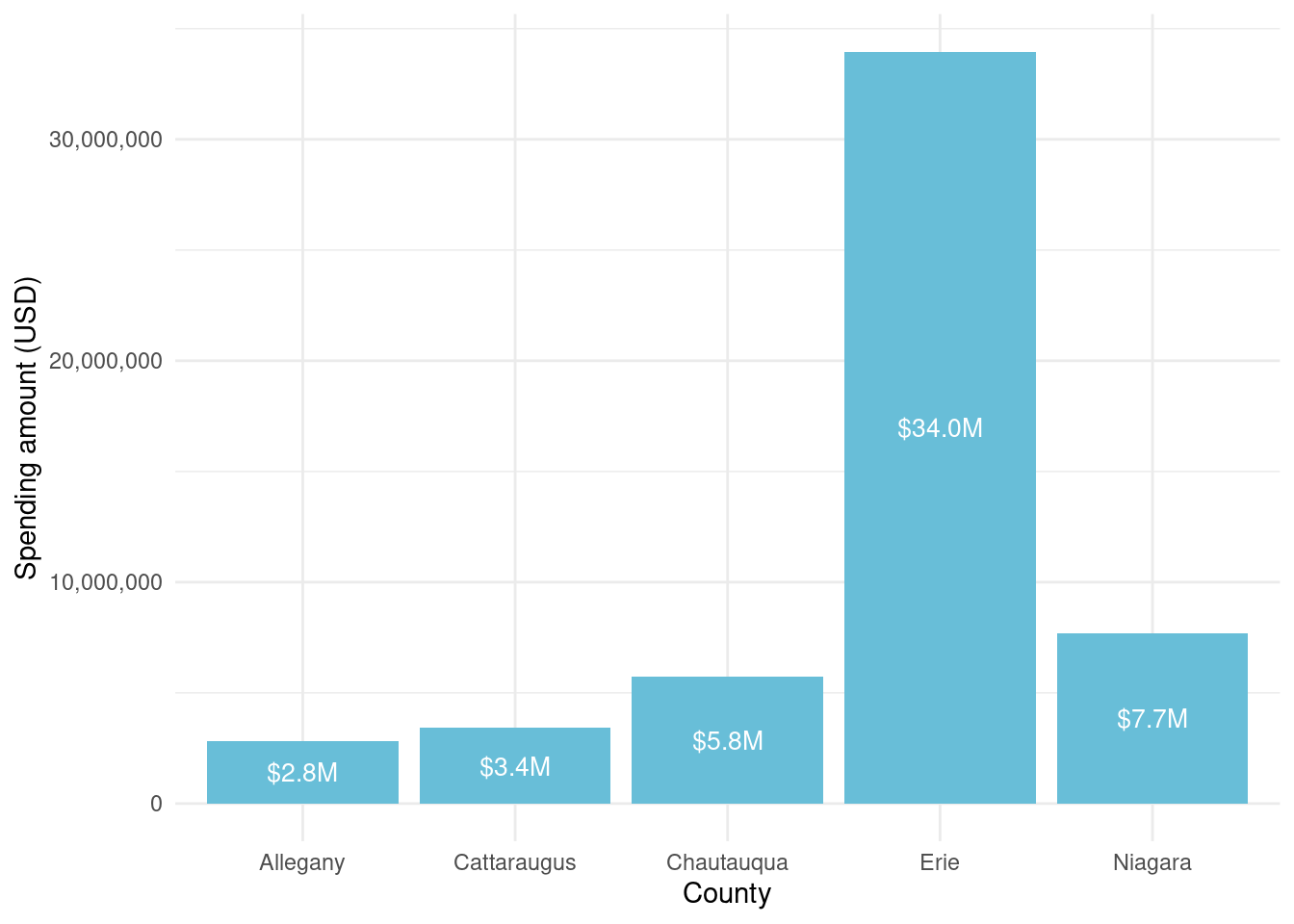
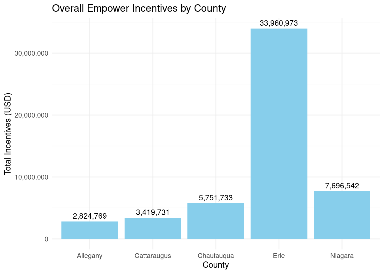
What was spent by county? - Allegany 2,824,769 - Cattaraugus 3,419,731 - Chautauqua 5,751,733 - Erie 33,960,973 - Niagara 7,696,542

As with Assisted, the majority of spending went to Erie County, which makes sense since it is the most populous.

What percent of potential beneficiaries benefitted?

In [53]:

county_lihh_wny <- zcta_hhlmi_wny |> 
  summarise(
    li_households = sum(li_households, na.rm = TRUE),
    .by = county
  )

In [54]:

county_totalstats_empower_wny <- county_lihh_wny |> 
  inner_join(county_projectstats_empower_wny, 
    by = join_by(county), 
    relationship = "one-to-one", 
    unmatched = "error"
    )

county_totalstats_empower_wny <- county_totalstats_empower_wny |> 
  mutate(
    beneficiary_hh_pct  = (total_projects / li_households) * 100,
    incentives_per_beneficiary = (total_incentives / total_projects)
  )

In [55]:

region_beneficiaries_empower_wny <- county_totalstats_empower_wny |>
  mutate(region_beneficiary_hh_pct = sum(total_projects) / sum(li_households))

In [56]:

county_projectstats_empower_wny |>
  ggplot(aes(x = county, y = total_incentives)) +
  geom_bar(stat = "identity", fill = sky) +
  geom_text(
    aes(label = paste0("$", scales::comma(total_incentives/1000000, accuracy = 0.1), "M")), 
    position = position_stack(vjust = 0.5), 
    color = "white", 
    size = 3.5
  ) +
  scale_y_continuous(labels = scales::comma) + 
  labs(
    x = "County",
    y = "Spending amount (USD)",
    fill = "Category"
  ) +
  theme_minimal()

In [57]:

In [58]:

county_projectstats_empower_wny |>
  mutate(across(where(is.numeric), scales::label_comma())) |>
  mutate(across(c("total_incentives", "total_bill_savings", "total_energy_savings"), function(x) paste0("$", as.character(x)))) |>
  knitr::kable(col.names = c("County",
                           "Projects count",
                           "Total incentives",
                           "Total bill savings",
                           "Total out-of-pocket spending"))

Empower program by the number by county

County	Projects count	Total incentives	Total bill savings	Total out-of-pocket spending
Chautauqua	885	$5,751,733	$411,737	$523,777
Erie	5,774	$33,960,973	$2,011,215	$2,275,455
Niagara	1,203	$7,696,542	$476,971	$435,002
Allegany	404	$2,824,769	$211,219	$237,170
Cattaraugus	527	$3,419,731	$276,561	$392,723

Percent of beneficiaries that benefitted by county: By county? - Allegany: 5.43% - Cattaraugus: 3.75% - Chautauqua: 3.51% - Erie: 3.43% - Niagara: 3.15%

Allegany has a somewhat higher percent of beneficiaries benefitted than other counties. This is in contrast to Assisted, which reached a 4-5x higher share of the eligible population in Erie and Niagara counties.

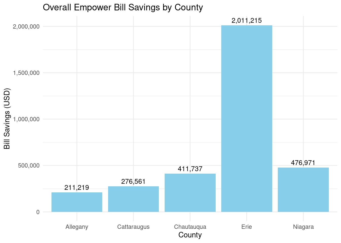
How many bill savings? Overall: $3,387,703 By county?

Allegany: 211,219
Cattaraugus: 276,561
Chautauqua: 411,737
Erie: 2,011,215
Niagara: 476,971

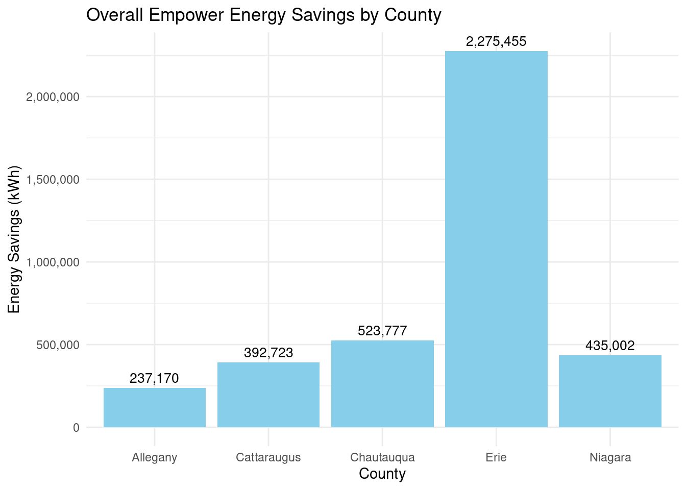
How many energy savings?

Overall: 3,864,127 kWh By county?

Allegany: 237,170
Cattaraugus: 392,723
Chautauqua: 523,777
Erie: 2,275,455
Niagara: 435,002

Graph showing overall incentives by county:

In [59]:

county_totalstats_empower_wny |> 
  ggplot(aes(x = county, y = total_incentives)) +
  geom_bar(stat = "identity", fill = "skyblue") +  
  geom_text(aes(label = scales::comma(total_incentives)), 
            vjust = -0.5, 
            color = "black", 
            size = 3.5) + 
  scale_y_continuous(labels = scales::comma) + 
  labs(title = "Overall Empower Incentives by County",
       x = "County",
       y = "Total Incentives (USD)") +
  theme_minimal() +
  theme(legend.position = "none")

Graph showing overall bill savings by county:

In [60]:

county_totalstats_empower_wny |>
ggplot(aes(x = county, y = total_bill_savings)) +
  geom_bar(stat = "identity", fill = "skyblue") +
  geom_text(aes(label = scales::comma(total_bill_savings)), 
            vjust = -0.5, 
            color = "black", 
            size = 3.5) +
  scale_y_continuous(labels = scales::comma) + 
  labs(title = "Overall Empower Bill Savings by County",
       x = "County",
       y = "Bill Savings (USD)") +
  theme_minimal()

Graph showing overall energy savings by county:

In [61]:

county_totalstats_empower_wny |>
ggplot(aes(x = county, y = total_energy_savings)) +
  geom_bar(stat = "identity", fill = "skyblue") +
  geom_text(aes(label = scales::comma(total_energy_savings)), 
            vjust = -0.5, 
            color = "black", 
            size = 3.5) +
  scale_y_continuous(labels = scales::comma) + 
  labs(title = "Overall Empower Energy Savings by County",
       x = "County",
       y = "Energy Savings (kWh)") +
  theme_minimal()

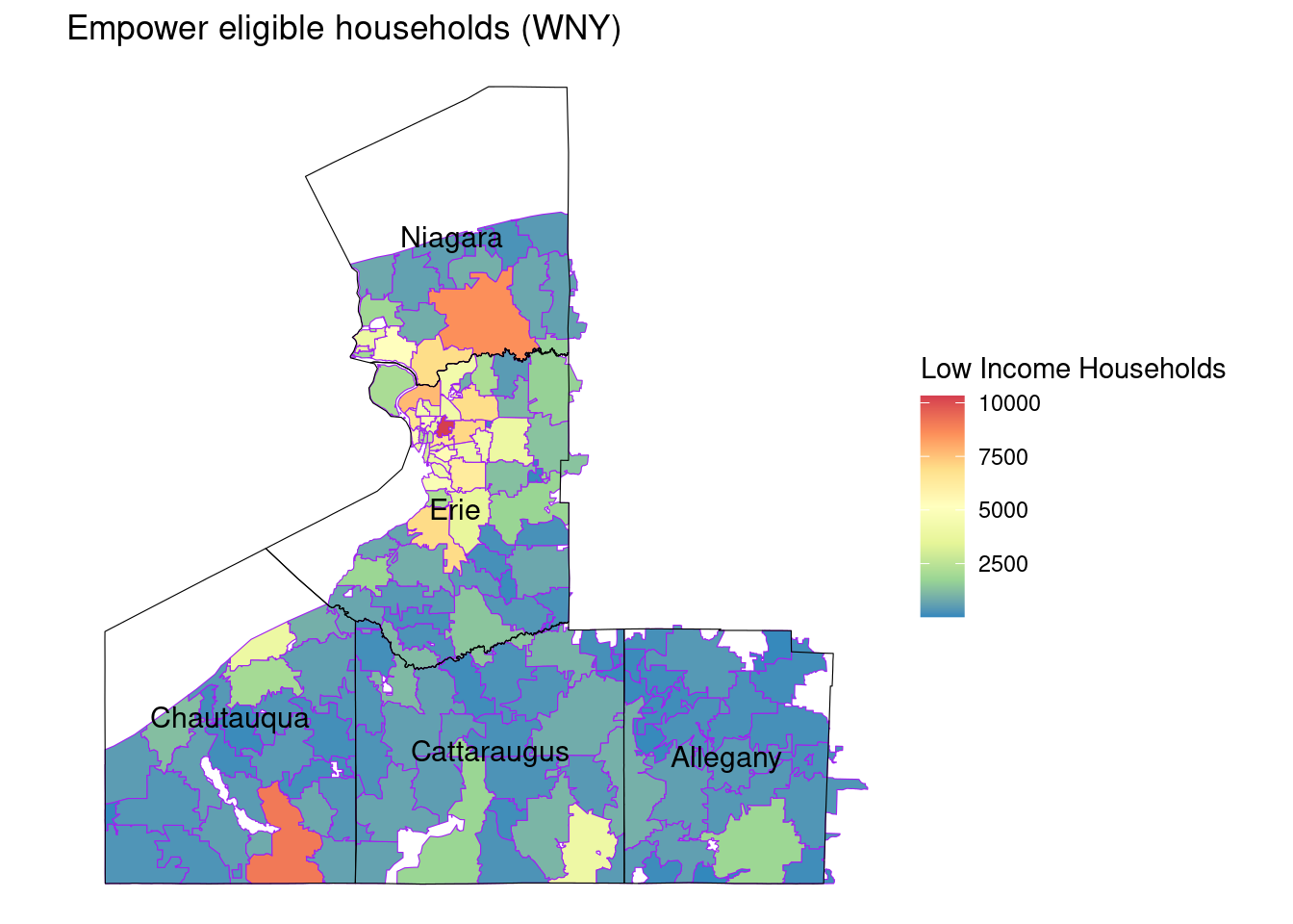
Geography

The data frame zcta_hhmi_wny_empower is created to show both hh level, income information and project level information. It is on the zcta level.

analysis by zcta:

In [62]:

zcta_hhli_wny <- zcta_hhlmi_wny |> 
  select(-c(mi_households, lmi_households, pct_mi, pct_lmi))

zcta_totalstats_empower_wny <- zcta_hhli_wny |> 
  right_join(zip_projectstats_empower_wny, 
    by = join_by(zcta == zip), 
1    relationship = "one-to-one"
  )  |> 
  filter(county != "NA")

1: For the right join here, we know it is working because every zip in zip_projectstats_empower_wny finds a match in zcta_hhli_wny. Our final df should have 147 rows as in zip_projectstats_empower_wny, which it does so we can proceed.

The df zcta_totalstats_bybeneficiary_empower_wny is created to get total incentives numbers and bill and energy savings, as well as spending/savings by empower beneficiary.

In [63]:

zcta_totalstats_bybeneficiary_empower_wny <- zcta_totalstats_empower_wny |>
  mutate(
    incentives_per_beneficiary_hh = total_incentives / total_projects, 
    billsavings_per_beneficiary_hh = total_bill_savings / total_projects, 
    energysavings_per_beneficiary_hh = total_energy_savings / total_projects,
    .keep = "used"
  )

Where are the potential beneficiaries? By county?

In [64]:

zcta_totalstats_empower_wny_geom <- left_join(zcta_totalstats_empower_wny,
  zcta_boundary_wny, 
  by = join_by(zcta == ZCTA5CE10), 
  relationship ="one-to-one"
  )

In [65]:

zcta_totalstats_empower_wny_sf <- st_as_sf(zcta_totalstats_empower_wny_geom)

Maps start here: showing all low income hh

In [66]:

zcta_totalstats_empower_wny_sf |>
  ggplot() +
    geom_sf(aes(fill = li_households), color = "purple") +
    geom_sf(data = county_boundary_wny, fill = NA, color = "black", size = 1) +  
    geom_sf_text(data = county_boundary_wny, 
                aes(label = NAME10), 
                size = 4, 
                color = "black") +  
    scale_fill_distiller(palette = "Spectral", 
                        name = "Low Income Households", 
                        direction = -1) +
    theme_void() +
    labs(title = "Empower eligible households (WNY)",
  )

Warning in st_point_on_surface.sfc(sf::st_zm(x)): st_point_on_surface may not
give correct results for longitude/latitude data

Normalized map: li hh / total hh

In [67]:

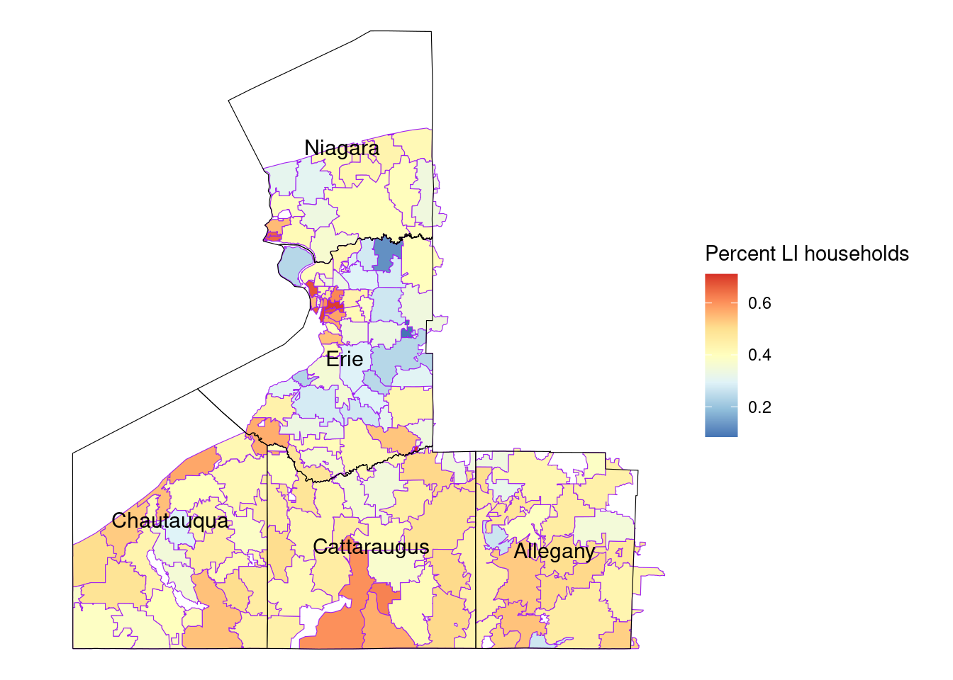
zcta_totalstats_empower_wny_sf |>
  ggplot() +
    geom_sf(aes(fill = li_households / total_households), color = "purple") +
    geom_sf(data = county_boundary_wny, fill = NA, color = "black", size = 1) +  
    geom_sf_text(data = county_boundary_wny, 
                aes(label = NAME10), 
                size = 4, 
                color = "black") +  
    scale_fill_distiller(palette = "RdYlBu", 
                        name = "Percent LI households") +
    theme_void()

Warning in st_point_on_surface.sfc(sf::st_zm(x)): st_point_on_surface may not
give correct results for longitude/latitude data

Percent Empower eligible households (WNY)

Cattaraugus, Chattauqua, and Allegany counties appear to have the highest percentages of LI households. Erie appears to have the most zcta-level variation in percent LI households.

Data analysis for geography related questions at the county starts here:

In [68]:

county_beneficiaries_empower_wny <- county_totalstats_empower_wny |> 
  mutate( 
    potential_beneficiaries = li_households,
    incentives_pct = (total_incentives / sum(total_incentives)) * 100,
    billsavings_per_beneficiary = total_bill_savings / total_projects, 
    energysavings_per_beneficiary = total_energy_savings / total_projects, 
    .keep = "unused"
  )

In [69]:

In [70]:

county_beneficiaries_empower_wny |>
  select(c(county, incentives_per_beneficiary)) |>
  mutate(across(where(is.numeric), scales::label_comma())) |>
  mutate(across(c("incentives_per_beneficiary"), function(x) paste0("$", as.character(x)))) |>
  knitr::kable()

Empower program incentives per beneficiary by county

county	incentives_per_beneficiary
Erie	$5,882
Niagara	$6,398
Cattaraugus	$6,489
Chautauqua	$6,499
Allegany	$6,992

In [71]:

In [72]:

county_beneficiaries_empower_wny |>
  select(c(county, potential_beneficiaries, beneficiary_hh_pct)) |>
  mutate(beneficiary_hh_pct = paste0(format(round(beneficiary_hh_pct, 2), nsmall = 2), "%")) |>
  mutate(across(where(is.numeric), scales::label_comma())) |>
  knitr::kable(col.names = c("County",
                            "Potential beneficiaries count",
                            "Subsidy recipients percentage"))

Empower program beneficiary percentage

County	Potential beneficiaries count	Subsidy recipients percentage
Erie	168,561	3.43%
Niagara	38,170	3.15%
Cattaraugus	14,072	3.75%
Chautauqua	25,249	3.51%
Allegany	7,436	5.43%

In [73]:

In [74]:

county_beneficiaries_empower_wny |>
  select(c(county, incentives_per_beneficiary, billsavings_per_beneficiary, energysavings_per_beneficiary)) |>
  mutate(across(where(is.numeric), scales::label_comma(accuracy = 1))) |>
  mutate(across(c("incentives_per_beneficiary", "billsavings_per_beneficiary"), function(x) paste0("$", as.character(x)))) |>
  knitr::kable(col.names = c("County",
                            "Incentives",
                            "Bill savings",
                            "Energy savings (kW)"))

Empower program measures per beneficiary by county

County	Incentives	Bill savings	Energy savings (kW)
Erie	$5,882	$348	394
Niagara	$6,398	$396	362
Cattaraugus	$6,489	$525	745
Chautauqua	$6,499	$465	592
Allegany	$6,992	$523	587

Where did this money go? By county: - Erie: 63.3%
- Niagara: 14.3%
- Chautauqua: 10.7% - Cattaraugus: 6.37% - Allegany: 5.26%

Money over beneficiaries? - Allegany 6992. - Cattaraugus 6489. - Chautauqua 6499. - Erie 5882. - Niagara 6398.

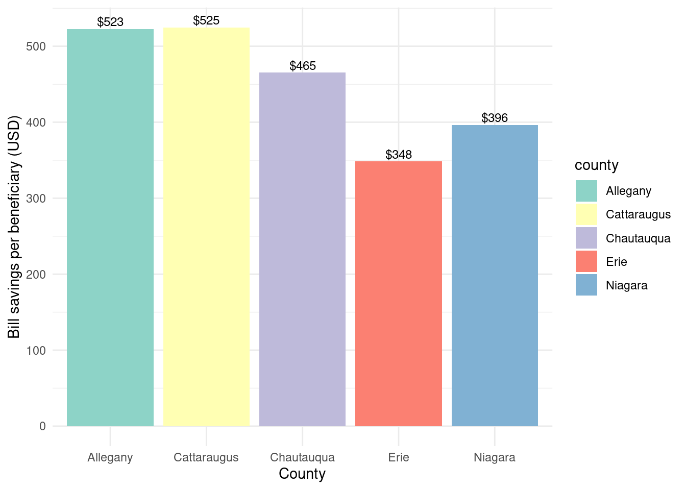
Bill savings over beneficiaries? - Allegany 523. - Cattaraugus 525. - Chautauqua 465. - Erie 348. - Niagara 396.

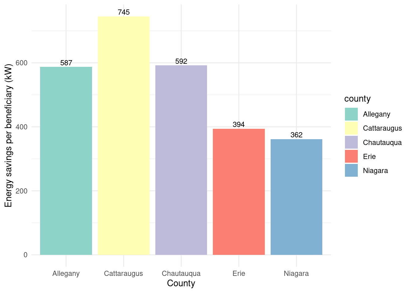
Energy savings over beneficiaries? - Allegany 587. - Cattaraugus 745. - Chautauqua 592. - Erie 394. - Niagara 362.

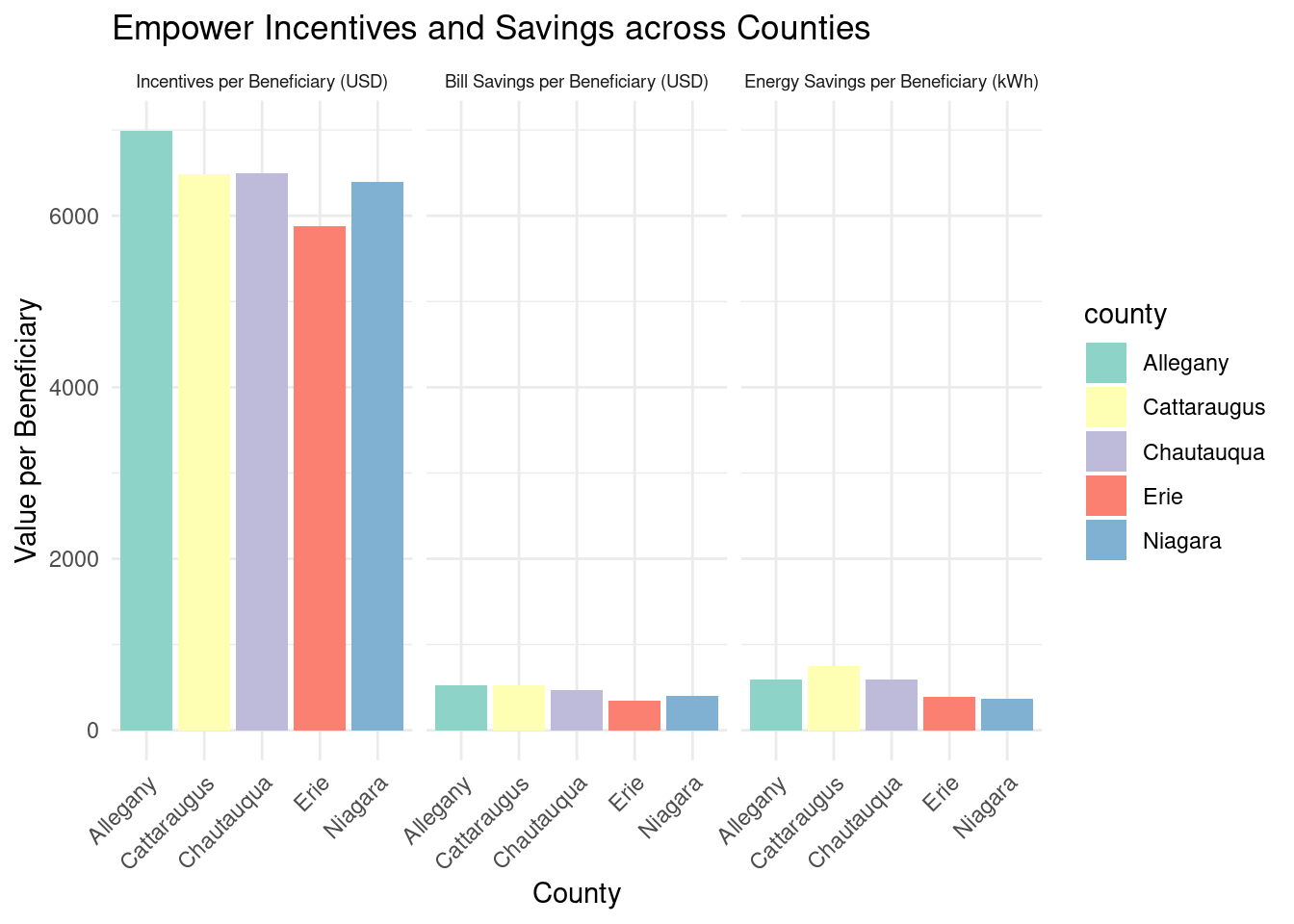
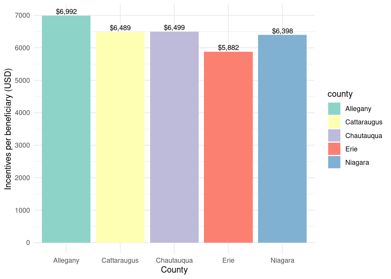
As with Assisted, for Empower Allegany had the highest incentive dollar amount per beneficiary. Cattaraugus, Chautauqua, and Niagara are fairly similar, while Erie had the lowest incentive dollar amount per benficiary. This means that Erie has the lowest incentive dollar amount per beneficiary, meaning that while the total allocation was high, it was spread across a larger number of beneficiaries. Allegany had the smallest percentage of money but had the highest incentive dollar amount per beneficiary. This suggests that fewer individuals received assistance, but the assistance per person was larger. Overall, a range of about 1k comparing the highest (Allegany) to the lowest (Erie).

Allegany and Chautauqua had somewhat higher bill savings over beneficiaries than other counties. Cattauraugus had the highest energy savings per beneficiary, followed by Chautauqua and Allegany.

The variation in energy savings per beneficiary could be explained by rural counties having higher energy bills (as with assisted).

Multiple bar graph showing spending/savings:

In [75]:

county_beneficiaries_empower_wny_long <- county_beneficiaries_empower_wny |>
  pivot_longer(
    cols = c(
      incentives_per_beneficiary, 
      billsavings_per_beneficiary, 
      energysavings_per_beneficiary
    ),
    names_to = "category",
    values_to = "value"
  ) |>
  mutate(
    category = factor(
      category, 
      levels = c(
        "incentives_per_beneficiary", 
        "billsavings_per_beneficiary", 
        "energysavings_per_beneficiary"
      )
    )
  )

In [76]:

empower_graph_label <- as_labeller(c(
  "incentives_per_beneficiary" = "Incentives per Beneficiary (USD)",
  "billsavings_per_beneficiary" = "Bill Savings per Beneficiary (USD)",
  "energysavings_per_beneficiary" = "Energy Savings per Beneficiary (kWh)"
))

In [77]:

county_beneficiaries_empower_wny_long |> 
ggplot(aes(x = county, y = value, fill = county)) +
  geom_bar(stat = "identity") +
  facet_wrap(~category, scales = "fixed", labeller = empower_graph_label) +
  labs(title = "Empower Incentives and Savings across Counties",
       x = "County",
       y = "Value per Beneficiary") +
  theme_minimal() +
  scale_fill_brewer(palette = "Set3") + 
  theme(axis.text.x = element_text(angle = 45, hjust = 1), 
  strip.text.x = element_text(size = 7))

In [78]:

county_beneficiaries_empower_wny |>
  ggplot(aes(x = county, y = incentives_per_beneficiary, fill = county)) +
  geom_bar(stat = "identity") +
  theme_minimal() +
  labs(x = "County",
      y = "Incentives per beneficiary (USD)") +
  geom_text(aes(label = paste0("$", scales::comma(incentives_per_beneficiary, accuracy = 1))),
          vjust = -0.3,
          color = "black",
          position = position_dodge(width = 0.9),
          size = 3.2) +
  scale_fill_brewer(palette = "Set3") +
  scale_y_continuous(breaks = seq(0, 10000, 1000))

Total incentives per beneficiary by county for Empower program

In [79]:

county_beneficiaries_empower_wny |>
  ggplot(aes(x = county, y = billsavings_per_beneficiary, fill = county)) +
  geom_bar(stat = "identity") +
  theme_minimal() +
  labs(x = "County",
      y = "Bill savings per beneficiary (USD)") +
  geom_text(aes(label = paste0("$", scales::comma(billsavings_per_beneficiary, accuracy = 1))),
          vjust = -0.3,
          color = "black",
          position = position_dodge(width = 0.9),
          size = 3.2) +
  scale_fill_brewer(palette = "Set3")

Bill savings per beneficiary by county for Empower program

In [80]:

county_beneficiaries_empower_wny |>
  ggplot(aes(x = county, y = energysavings_per_beneficiary, fill = county)) +
  geom_bar(stat = "identity") +
  theme_minimal() +
  labs(x = "County",
      y = "Energy savings per beneficiary (kW)") +
  geom_text(aes(label = scales::comma(energysavings_per_beneficiary, accuracy = 1)),
          vjust = -0.3,
          color = "black",
          position = position_dodge(width = 0.9),
          size = 3.2) +
  scale_fill_brewer(palette = "Set3")

Energy savings per beneficiary by county for Empower program

Race

overall first.

In [81]:

zcta_lihh_byrace_wny <- zctarace_hhlmi_wny |> 
  mutate(
    total_lihh = sum(li_households, na.rm = TRUE), # total_lihh by zcta
    .by = c(zcta, county)
  ) |>
  rename(lihh_by_race = li_households) |>
  select(-c(mi_households, 
            lmi_households, 
            total_households, 
            pct_li, 
            pct_mi,   
            pct_lmi)
  )

zcta_totalstats_empower_wny <- zip_projectstats_empower_wny |> 
  left_join(zcta_lihh_byrace_wny, 
    by = join_by(zip == zcta),
    relationship = "one-to-many",
  ) |> 
1  filter(county != "NA")

zcta_totalstats_empower_wny <- zcta_totalstats_empower_wny |>
  mutate(
    li_zcta_percent = lihh_by_race / total_lihh,
    empower_incentives_race = li_zcta_percent * total_incentives,
    empower_billsavings_race = li_zcta_percent * total_bill_savings,
    empower_energysavings_race = li_zcta_percent * total_energy_savings,
    empower_totalprojects_race = li_zcta_percent * total_projects,
    .by = c(zip, county)
  )

1: Each project in Empower project stats maps to zip in race data, resulting in a data frame of 147 * 5 = 735

In [82]:

region_totalstats_byrace_empower_wny <- zcta_totalstats_empower_wny |> 
  summarize(
    empower_incentives_race = sum(empower_incentives_race, 
      na.rm = TRUE),
    empower_billsavings_race = sum(empower_billsavings_race, 
      na.rm = TRUE),
    empower_energysavings_race = sum(empower_energysavings_race, 
      na.rm = TRUE),
    empower_totalprojects_race  = sum(empower_totalprojects_race,
      na.rm = TRUE),
    .by = race
  )

In [83]:

region_pctstats_byrace_empower_wny <- 
  region_totalstats_byrace_empower_wny |>
    mutate(
      empower_incentives_race = empower_incentives_race / 
        sum(empower_incentives_race) * 100,
      empower_billsavings_race = empower_billsavings_race /
        sum(empower_billsavings_race) * 100,
      empower_energysavings_race = empower_energysavings_race /
        sum(empower_energysavings_race) * 100,
      empower_totalprojects_race = empower_totalprojects_race /
        sum(empower_totalprojects_race) * 100
    )

What percent of beneficiaries are white vs. black vs. native vs. other? - white 72.7%
- black 18.8%
- native 0.682% - asian 2.22% - other 5.62%

What percent of spending went to white vs. black vs. native vs. other? - white 73.4%
- black 18.3%
- native 0.680% - asian 2.16% - other 5.49%

What percent of bill savings went to white vs. black vs. native vs. other? - white 73.6%
- black 18.2%
- native 0.688% - asian 2.12% - other 5.35%

What percent of energy savings went to white vs. black vs. native vs. other? - white 74.4
- black 17.6
- native 0.709 - asian 2.06 - other 5.22

By county?

In [84]:

county_totalstats_byrace_empower_wny <- zcta_totalstats_empower_wny |> 
  summarize(
    empower_incentives_race = sum(empower_incentives_race, 
      na.rm = TRUE),
    empower_billsavings_race = sum(empower_billsavings_race, 
      na.rm = TRUE),
    empower_energysavings_race = sum(empower_energysavings_race, 
      na.rm = TRUE),
    empower_totalprojects_race = sum(empower_totalprojects_race,
      na.rm = TRUE),
    empower_totalhouseholds_race = sum(lihh_by_race, na.rm = TRUE),
    .by = c(county, race)
  )

The df wny_project_li_race_hh_empower_spending is then created to get spending by household by race.

In [85]:

region_incentives_byrace_empower_wny <- 
  county_totalstats_byrace_empower_wny |>
    summarize(
      total_incentives = sum(empower_incentives_race),
      total_potential_beneficiaries = sum(empower_totalhouseholds_race),
      .by = race) |>
    mutate(
      incentives_per_potential_beneficiary = total_incentives / total_potential_beneficiaries
  )

Graph showing race spending (Overall WNY)

In [86]:

region_incentives_byrace_empower_wny |>
  ggplot(aes(x = race, y = incentives_per_potential_beneficiary, fill = race)) +
  geom_text(aes(label = scales::comma(incentives_per_potential_beneficiary, accuracy = 0.01)),
            vjust = -0.3,
            color = "black",
            position = position_dodge(width = 0.9),
            size = 3.2) +
  geom_bar(stat = "identity") +
  labs(title = "Empower Incentives per Household by Race for WNY",
       x = "Race",
       y = "Incentives per Beneficiary Household (USD)") +
  theme_minimal() +
  scale_fill_brewer(palette = "Set3")

As with Assisted, for Empower Black households appear to hae received the highest spending per household.

Based on our analysis, this could imply that more racially diverse ZCTAs received more funding.

county_totalstats_byrace_assisted_wny is also used to get a df that shows percent spending/savings

In [87]:

county_pctstats_byrace_empower_wny <- 
  county_totalstats_byrace_empower_wny |>
    mutate(
      incentives_total = sum(empower_incentives_race, 
        na.rm = TRUE),
      billsavings_total = sum(empower_billsavings_race,
        na.rm = TRUE),
      energysavings_total = 
        sum(empower_energysavings_race, na.rm = TRUE), 
      totalprojects_total = 
        sum(empower_totalprojects_race, na.rm = TRUE),
      .by = county
    ) |> 
    mutate(
      incentives_byrace_pct = empower_incentives_race /
        incentives_total * 100,
      billsavings_byrace_pct = empower_billsavings_race /
        billsavings_total * 100,
      energysavings_byrace_pct = 
        empower_energysavings_race / energysavings_total  
          * 100,
      totalprojects_byrace_pct = 
        empower_totalprojects_race / 
        totalprojects_total * 100,
      .keep = "unused"
    ) |>
    select(-c(empower_totalhouseholds_race) # irrelevant variable
    )

What percent of beneficiaries are white vs. black vs. native vs. other? 1 Allegany white 98.2
2 Allegany black 0.237 3 Allegany native 0.486 4 Allegany asian 0.0603 5 Allegany other 1.05
6 Cattaraugus white 93.2
7 Cattaraugus black 1.37
8 Cattaraugus native 2.06
9 Cattaraugus asian 0.511 10 Cattaraugus other 2.87
11 Chautauqua white 91.8
12 Chautauqua black 2.41
13 Chautauqua native 0.361 14 Chautauqua asian 0.580 15 Chautauqua other 4.86
16 Erie white 64.1
17 Erie black 25.8
18 Erie native 0.555 19 Erie asian 3.05
20 Erie other 6.53
21 Niagara white 83.2
22 Niagara black 10.6
23 Niagara native 1.01
24 Niagara asian 0.804 25 Niagara other 4.47

What percent of spending went to white vs. black vs. native vs. other? 1 Allegany white 98.2
2 Allegany black 0.236 3 Allegany native 0.504 4 Allegany asian 0.0590 5 Allegany other 1.04
6 Cattaraugus white 93.3
7 Cattaraugus black 1.32
8 Cattaraugus native 2.02
9 Cattaraugus asian 0.491 10 Cattaraugus other 2.84
11 Chautauqua white 92.1
12 Chautauqua black 2.30
13 Chautauqua native 0.324 14 Chautauqua asian 0.507 15 Chautauqua other 4.75
16 Erie white 64.1
17 Erie black 25.8
18 Erie native 0.553 19 Erie asian 3.09
20 Erie other 6.46
21 Niagara white 83.1
22 Niagara black 10.6
23 Niagara native 0.992 24 Niagara asian 0.772 25 Niagara other 4.49

What percent of bill savings went to white vs. black vs. native vs. other? 1 Allegany white 98.2
2 Allegany black 0.218 3 Allegany native 0.476 4 Allegany asian 0.0661 5 Allegany other 1.03
6 Cattaraugus white 93.7
7 Cattaraugus black 1.31
8 Cattaraugus native 1.68
9 Cattaraugus asian 0.465 10 Cattaraugus other 2.88
11 Chautauqua white 92.8
12 Chautauqua black 2.08
13 Chautauqua native 0.328 14 Chautauqua asian 0.529 15 Chautauqua other 4.32
16 Erie white 62.1
17 Erie black 27.5
18 Erie native 0.567 19 Erie asian 3.19
20 Erie other 6.61
21 Niagara white 83.9
22 Niagara black 10.0
23 Niagara native 1.04
24 Niagara asian 0.789 25 Niagara other 4.20

What percent of energy savings went to white vs. black vs. native vs. other? 1 Allegany white 98.2
2 Allegany black 0.312 3 Allegany native 0.550 4 Allegany asian 0.0591 5 Allegany other 0.920 6 Cattaraugus white 93.7
7 Cattaraugus black 1.01
8 Cattaraugus native 1.95
9 Cattaraugus asian 0.363 10 Cattaraugus other 3.01
11 Chautauqua white 93.1
12 Chautauqua black 1.89
13 Chautauqua native 0.342 14 Chautauqua asian 0.556 15 Chautauqua other 4.07
16 Erie white 63.0
17 Erie black 26.9
18 Erie native 0.541 19 Erie asian 3.13
20 Erie other 6.41
21 Niagara white 82.2
22 Niagara black 11.4
23 Niagara native 1.03
24 Niagara asian 0.762 25 Niagara other 4.67

In [88]:

county_spending_byrace_empower_wny <- county_totalstats_byrace_empower_wny |>
  rename(
      total_incentives = empower_incentives_race,
      total_beneficiaries = empower_totalprojects_race,
    ) |>
    mutate(
      spending_per_beneficiary = total_incentives / total_beneficiaries,
    ) |>
    select(c(county, race, total_incentives, total_beneficiaries, spending_per_beneficiary))

county_spending_byrace_empower_wny <- 
county_totalstats_byrace_empower_wny |>
    summarize(
      total_spending_by_race = sum(empower_incentives_race),
      total_race_hh = sum(empower_totalhouseholds_race),
      .by = c(race, county)) |>
    mutate(
      spending_per_hh_by_race = total_spending_by_race / total_race_hh
  )

Graph showing race spending (By county)

In [89]:

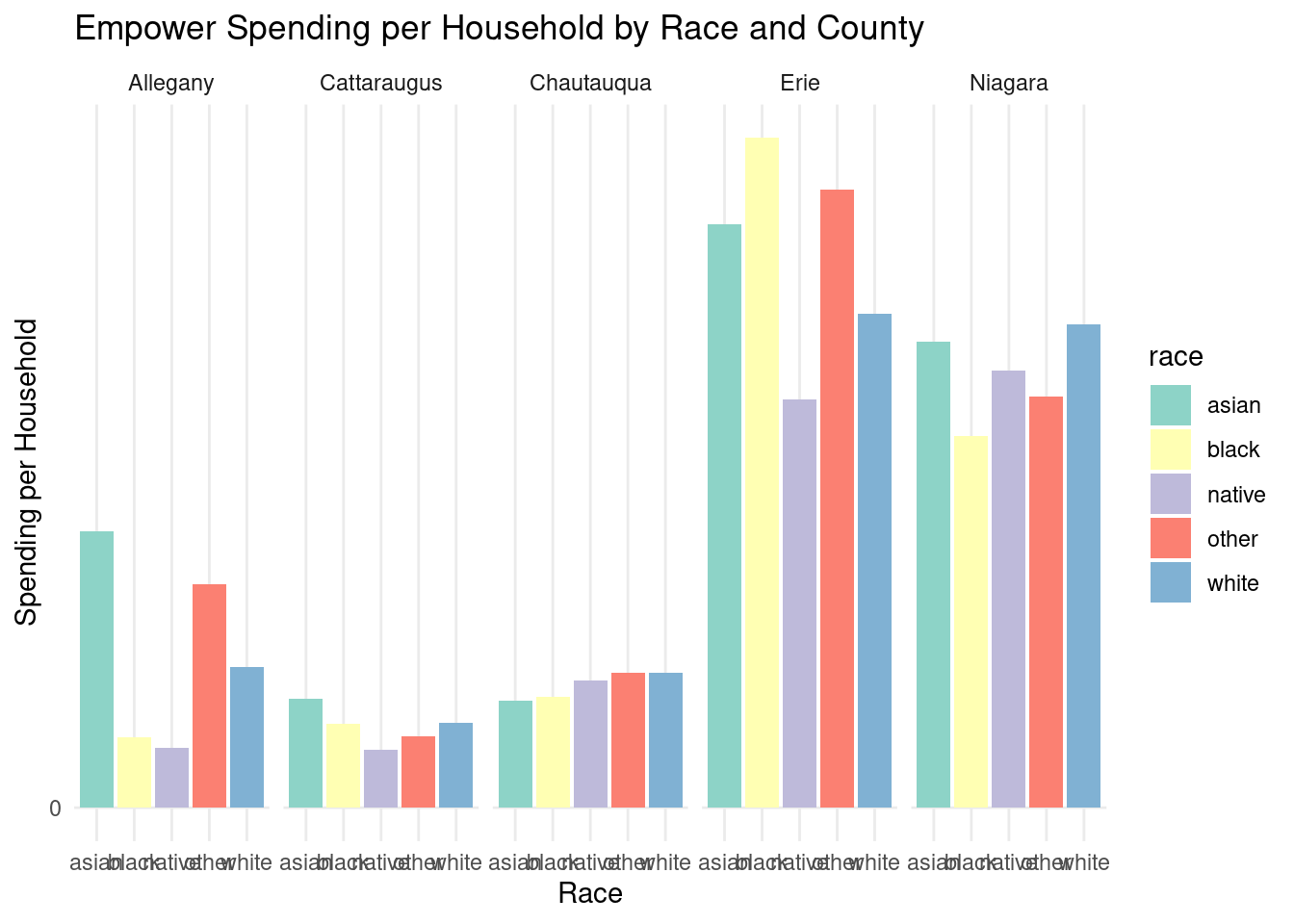
county_spending_byrace_assisted_wny |>
  ggplot(aes(x = race, y = spending_per_potential_beneficiary, fill = race)) +
  geom_bar(stat = "identity") +
  labs(
    title = "Empower Spending per Household by Race and County",
    x = "Race",
    y = "Spending per Household"
  ) +
  scale_y_continuous(labels = scales::comma, breaks = seq(0, 15000, 2500)) +
  theme_minimal() +
  scale_fill_brewer(palette = "Set3") +
  facet_grid(~county)

In [90]:

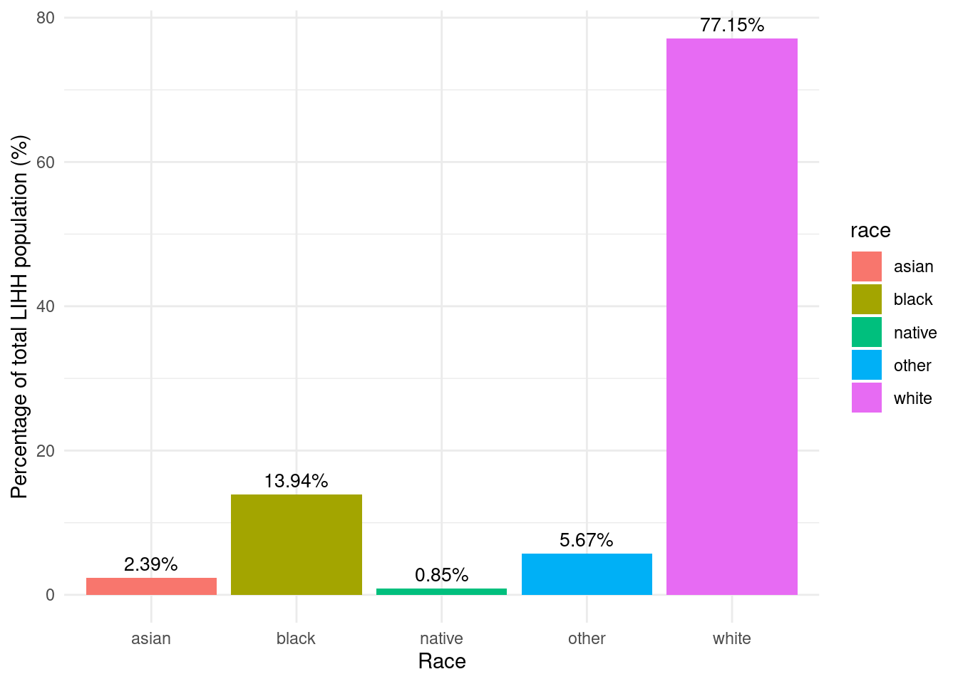
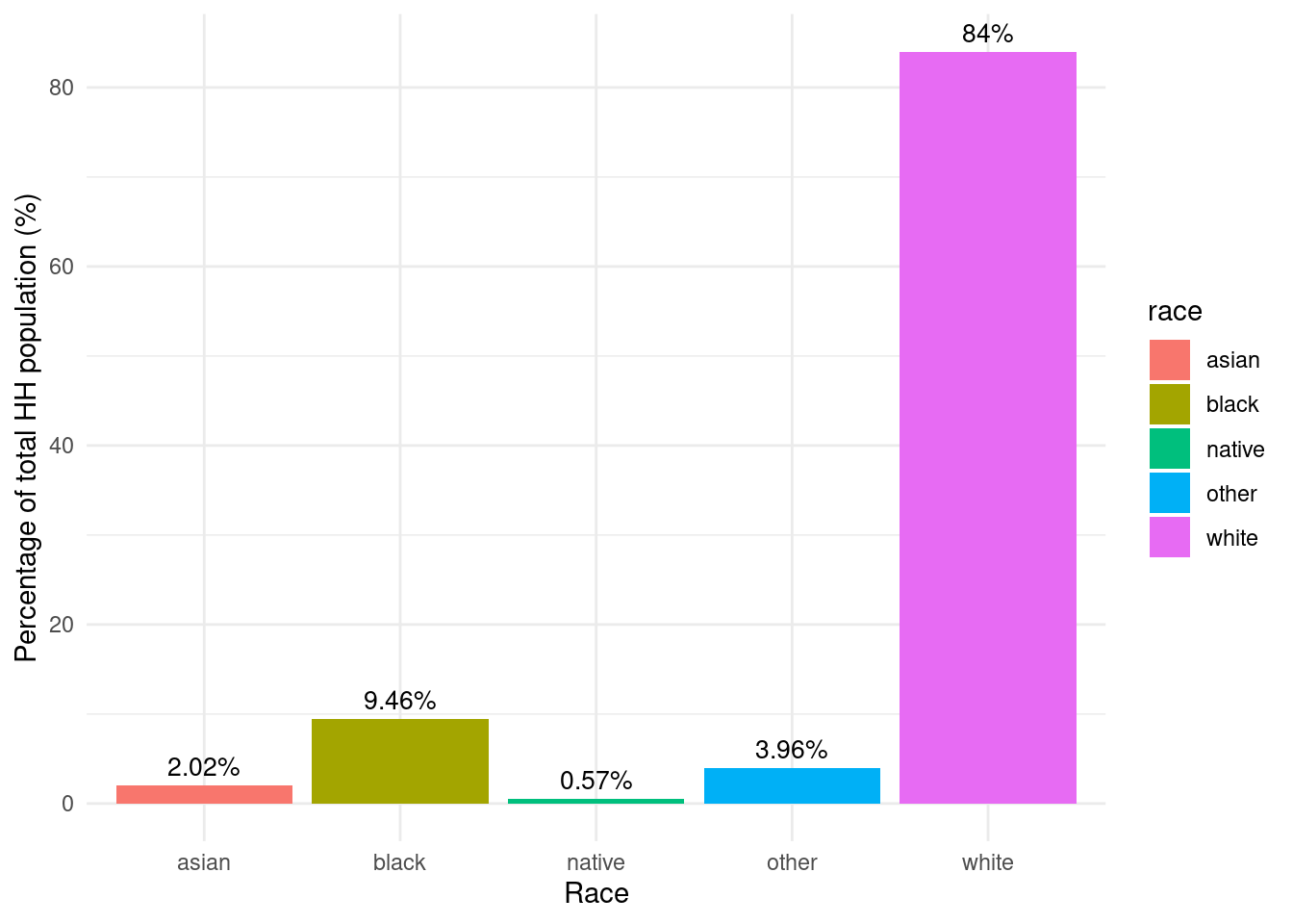
region_incentives_byrace_empower_wny |>
  mutate(lihh_pct = (total_potential_beneficiaries / sum(total_potential_beneficiaries)) * 100) |>
  mutate(lihh_pct = as.numeric(format(round(lihh_pct, 2), nsmall = 2))) |>
  ggplot(aes(y = lihh_pct, x = race, fill = race)) +
  labs(y = "Percentage of total LIHH population (%)",
  x = "Race") +
  geom_bar(stat = "identity") +
  geom_text(aes(label = paste0(lihh_pct, "%")), 
          vjust = -0.5, 
          color = "black", 
          size = 3.5) +
  theme_minimal()

Racial makeup of low income households in WNY

In [91]:

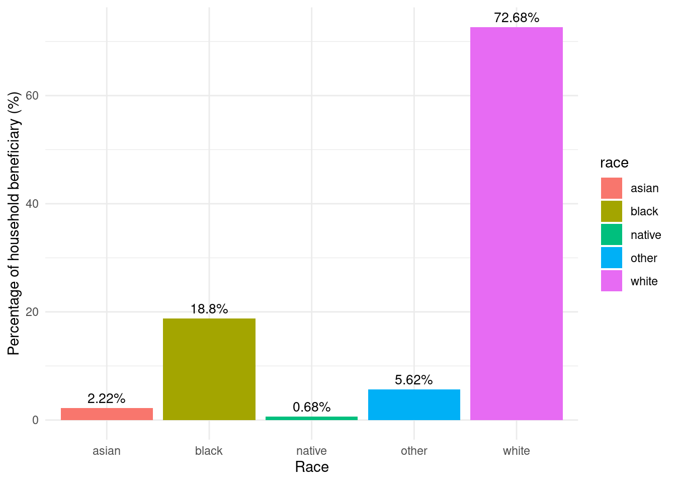
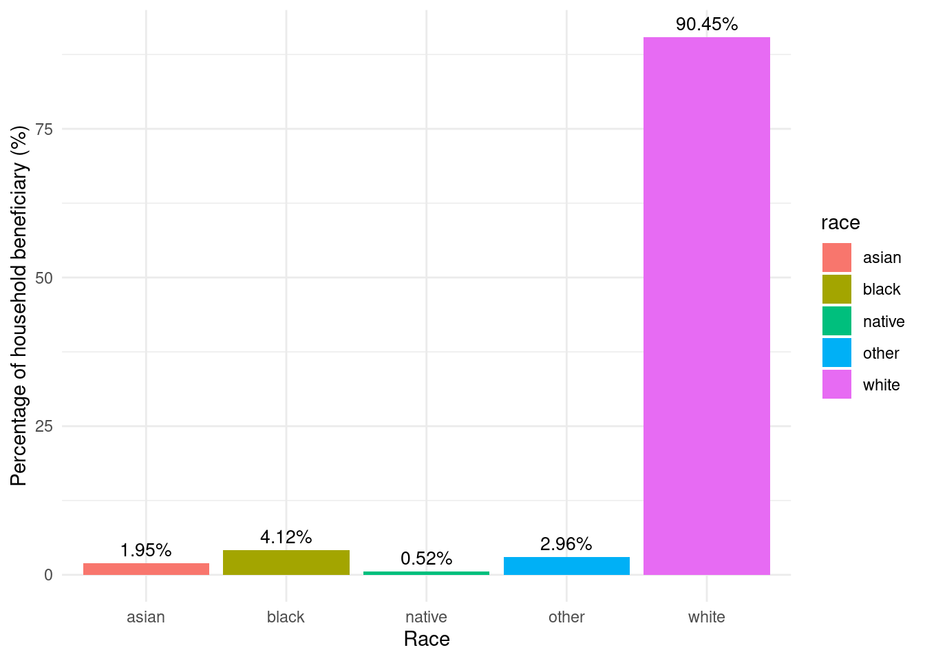
region_totalstats_byrace_empower_wny |>
  mutate(beneficiary_pct = (empower_totalprojects_race / sum(empower_totalprojects_race)) * 100) |>
  mutate(beneficiary_pct = as.numeric(format(round(beneficiary_pct, 2), nsmall = 2))) |>
  ggplot(aes(y = beneficiary_pct, x = race, fill = race)) +
  labs(y = "Percentage of household beneficiary (%)",
  x = "Race") +
  geom_bar(stat = "identity") +
  geom_text(aes(label = paste0(beneficiary_pct, "%")), 
          vjust = -0.5, 
          color = "black", 
          size = 3.5) +
  theme_minimal()

Racial makeup of Empower program’s beneficiary households in WNY

Counties vary in terms of the racial demographics of Empower spending by household. Some of this analysis may be complicated by the small amount of data available for some smaller counties. Estimates for Empower spending by race are probably less accurate by county than for Western NY overall.

Black households receive the highest levels of spending per household for both Allegany and Erie counties, as well as in Niagara (though this is a very slight difference).

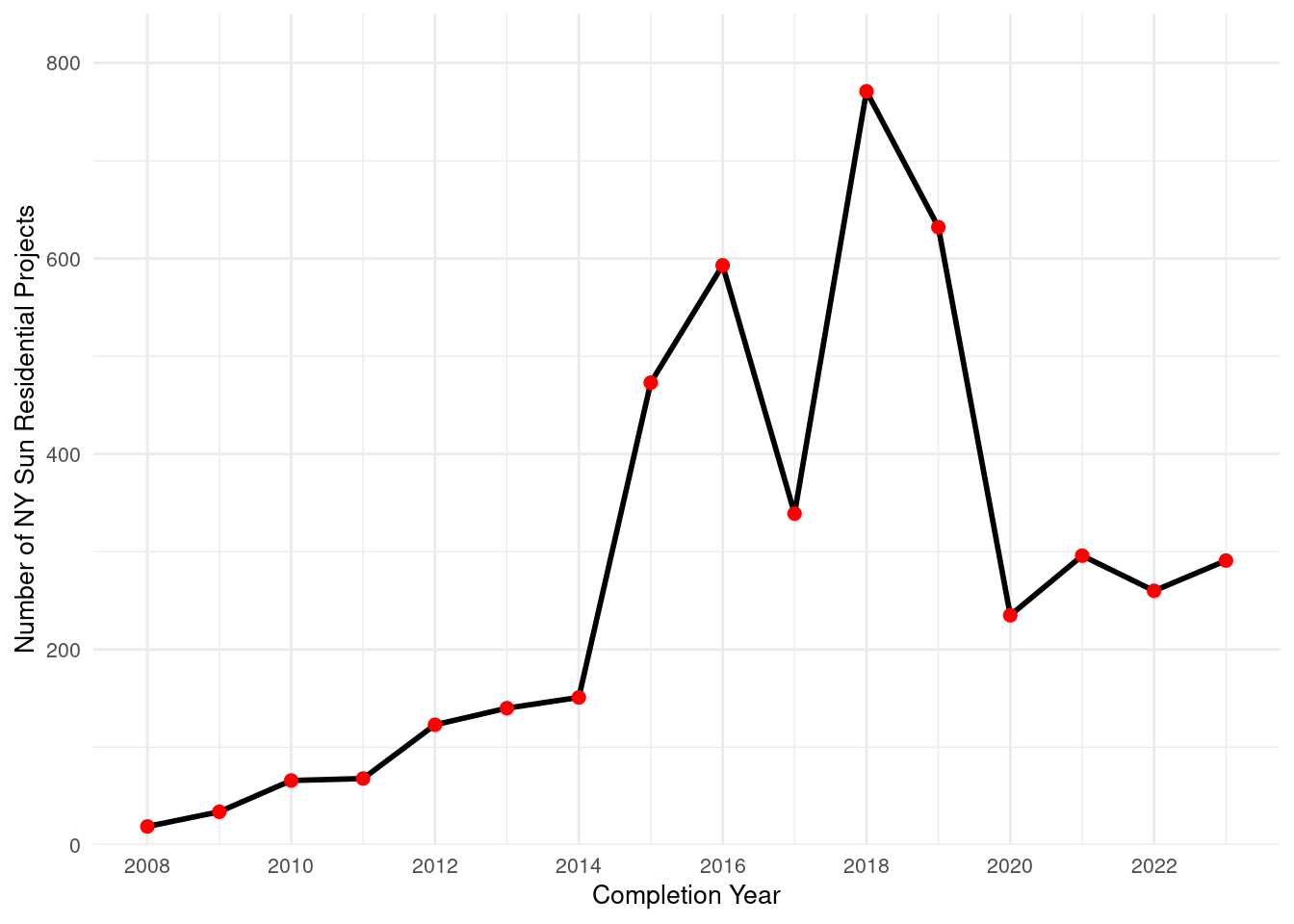
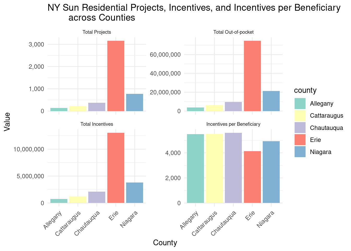
NY Sun Residential

The df region_projectstats_nysun_res_wny was created to show the overall number of projects, incentives, energy capacity, and energy generation in all of WNY.

One important thing to note for NYSun is that there are no income requirements. It can be applied to all households even if they are not lmi.

In [92]:

region_projectstats_nysun_res_wny <- county_projectstats_nysun_resi_wny |> 
  summarize_if(is.numeric, sum, na.rm=TRUE)

The df wny_countystats_nysunresi was created to show the overall number of projects, incentives, energy capacity, and energy generation by county in WNY.

Overall, there were 4,662 projects for Western NY during this time period.

Big picture

Let’s drill in on the years 2008-2023.

In [93]:

projects_nysun_resi_wny_08_23 <- projects_nysun_resi |>
  filter(county %in% wny_counties) |> 
  mutate(completion_year = year(project_completion_date)) |>
1  filter(!is.na(completion_year)) |>
2  filter(completion_year > 2007 & completion_year < 2024)

1: Some of the projects have not yet been completed which is why those have been filtered out.
2: Earlier years have also been filtered out because few projects were completed during that time. We also filtered out 2024 since the year is not over.

How much money was spent overall in WNY?

In [94]:

resi_wny_08_23_total_incentives <- projects_nysun_resi_wny_08_23 |> 
  summarize(sum(incentives, na.rm = TRUE))
  
resi_wny_08_23_total_incentives

# A tibble: 1 × 1
  `sum(incentives, na.rm = TRUE)`
                            <dbl>
1                       20360432.

Answer: $20,360,432

On how many projects?

In [95]:

resi_wny_08_23_total_projects <- projects_nysun_resi_wny_08_23 |>
 summarize(n())
  
resi_wny_08_23_total_projects

# A tibble: 1 × 1
  `n()`
  <int>
1  4491

Answer: 4,491.

Average spending per project?

In [96]:

resi_wny_08_23_total_incentives / resi_wny_08_23_total_projects

  sum(incentives, na.rm = TRUE)
1                      4533.608

$4,533

How much private investment did that catalyze?

In [97]:

projects_nysun_resi_wny_08_23 |> 
  summarize(sum(project_cost - incentives, na.rm = TRUE))

# A tibble: 1 × 1
  `sum(project_cost - incentives, na.rm = TRUE)`
                                           <dbl>
1                                     110362193.

Answer: $110,362,193

How much data total project cost data is missing?

In [98]:

projects_nysun_resi_wny_08_23 |> 
  mutate(
    project_cost_zero = project_cost == 0,
    project_cost_missing = is.na(project_cost)
  ) |> 
  summarize(
    sum(project_cost_missing) / n(),
    sum(project_cost_zero) / n(),
  )

# A tibble: 1 × 2
  `sum(project_cost_missing)/n()` `sum(project_cost_zero)/n()`
                            <dbl>                        <dbl>
1                               0                     0.000668

Almost none, so we use this figure.

How much solar capacity did that add?

In [99]:

projects_nysun_resi_wny_08_23 |> 
  summarize(sum(energy_capacity, na.rm = TRUE))

# A tibble: 1 × 1
  `sum(energy_capacity, na.rm = TRUE)`
                                 <dbl>
1                               36862.

36,862 kW, or 36 mW.

What is the average capacity per project?

In [100]:

projects_nysun_resi_wny_08_23 |> 
  summarize(sum(energy_capacity, na.rm = TRUE) / n())

# A tibble: 1 × 1
  `sum(energy_capacity, na.rm = TRUE)/n()`
                                     <dbl>
1                                     8.21

8.21 kW

How much of the solar capacity data is missing?

In [101]:

projects_nysun_resi_wny_08_23 |> 
  mutate(
    energy_capacity_zero = energy_capacity == 0,
    energy_capacity_missing = is.na(energy_capacity)
  ) |> 
  summarize(
    sum(energy_capacity_missing) / n(),
    sum(energy_capacity_zero) / n(),
  )

# A tibble: 1 × 2
  `sum(energy_capacity_missing)/n()` `sum(energy_capacity_zero)/n()`
                               <dbl>                           <dbl>
1                                  0                               0

None, so we can use the data.

Projects completed over time?

In [102]:

region_projectcountbyyear_nysun_res_wny <- projects_nysun_resi_wny_08_23 |>
  summarize(
    project_count_by_year = n(),
    .by = completion_year
  )

The scatterplot below shows the projects completed over time:

In [103]:

region_projectcountbyyear_nysun_res_wny |> 
  ggplot(
    aes(x = completion_year, y = project_count_by_year, group = 1)
  ) +
    geom_line(color = "black", linewidth = 1) +
    geom_point(color = "red", size = 2) +
    scale_x_continuous(breaks = seq(2008, 2023, 2)) +
    scale_y_continuous(breaks = seq(0, 800, 200), limit = c(0, 850), expand = c(0, NA)) +
    labs(x = "Completion Year",
      y = "Number of NY Sun Residential Projects"
  ) +
    theme_minimal() +
    theme(
      plot.title = element_text(size = 14, face = "bold"),
      axis.title = element_text(size = 10),
      axis.text = element_text(size = 8),
      plot.caption = element_text(size = 8, hjust = 1)
  )

Number of completed NY Sun Residential projects by year

The main year-to-year decrease occurred between 2016-2017, and then again a sharp decrease in 2020- perhaps due to the pandemic.

Money spent by county? In desc order:

1 Erie 13,052,190. 2 Niagara 3,831,428. 3 Chautauqua 2,101,823 4 Cattaraugus 1,211,624. 5 Allegany 731,419.

The most money for NY Sun Residential was spent in Erie county.

How much energy capacity? (kw) By county? In desc order:

1 Erie 24524 2 Niagara 7272. 3 Chautauqua 3237. 4 Cattaraugus 2122. 5 Allegany 1312.

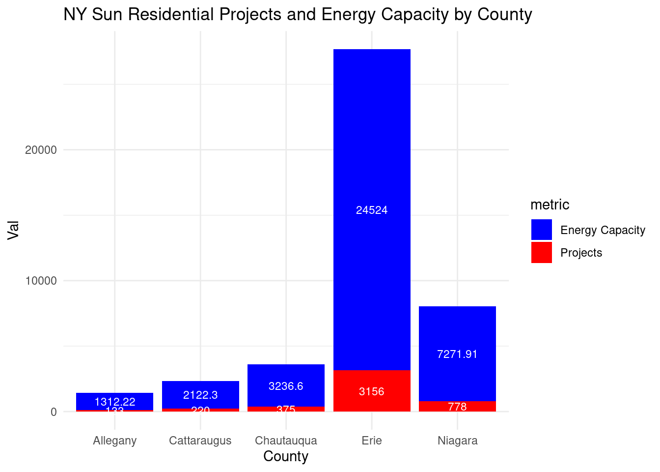
It seems like the incentives might be influencing the energy capacity generated by county. This could be because greater incentives = greater amt of projects.

Checking: Yes, if we look at amt of projects in desc order, it stays the same: 1 Erie 3156 2 Niagara 778 3 Chautauqua 375 4 Cattaraugus 220 5 Allegany 133

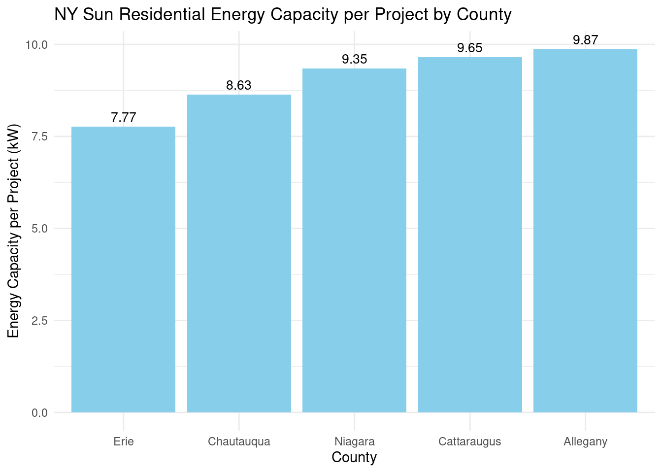
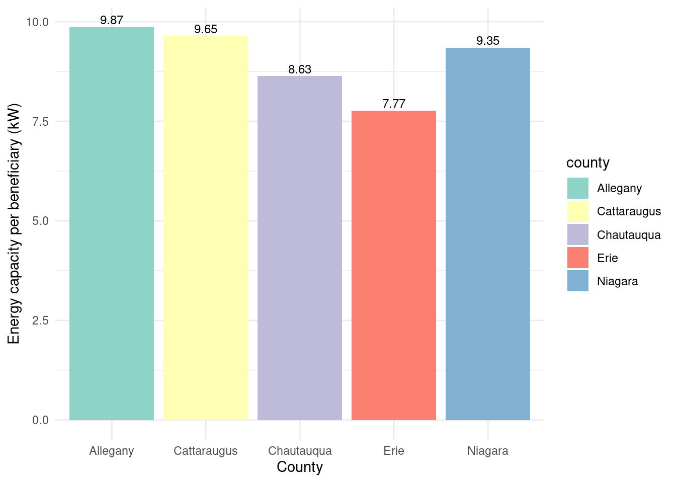
Looks like per project the amount of kw in energy capacity generated was:

In [104]:

# add incentives per beneficiary and rename df to county_projectstats_bybeneficiary_nysun_res_wny? 
county_avgcap_nysun_res_wny <- county_projectstats_nysun_resi_wny |>
mutate(avg_energy_capacity = total_energy_capacity / total_projects,
avg_energy_generation = total_energy_generation / total_projects,
avg_incentives = total_incentives / total_projects)

1 Allegany 9.87 2 Cattaraugus 9.65 3 Niagara 9.35 4 Chautauqua 8.63 5 Erie 7.77

Interestingly, the order here now reverses. is this expected? ^Potential question for further analysis - maybe counties with more projects had greater mix of small and large projects?TODO

Graph showing energy capacity and projects by county:

In [105]:

county_avgcap_nysun_res_wny_long <- 
pivot_longer(county_avgcap_nysun_res_wny, 
              cols = c(total_projects, total_energy_capacity), 
              names_to = "metric", values_to = "value")

In [106]:

# TODO: what is this graph saying??
county_avgcap_nysun_res_wny_long |> 
  ggplot(aes(x = county, y = value, fill = metric)) +
    geom_bar(stat = "identity", position = "stack") +
    geom_text(aes(label = value, 
                  size = ifelse(metric == "overall_projects", 3, 3)), 
              position = position_stack(vjust = 0.5), color = "white") +
    scale_size_identity() + 
    scale_fill_manual(values = c("total_projects" = "red", 
                                 "total_energy_capacity" = "blue"),
                      labels = c("total_projects" = "Projects", 
                                 "total_energy_capacity" = 
                                  "Energy Capacity")) +
    labs(title = "NY Sun Residential Projects and Energy Capacity by County", 
         x = "County", y = "Val") +
    theme_minimal()

In [107]:

county_avgcap_nysun_res_wny |> 
  ggplot(aes(x = reorder(county, avg_energy_capacity),
              y = avg_energy_capacity)) +
    geom_bar(stat = "identity", fill = "skyblue") +
    geom_text(aes(label = scales::comma(avg_energy_capacity)), 
          vjust = -0.5, 
          color = "black", 
          size = 3.5) + 
    labs(title = "NY Sun Residential Energy Capacity per Project by County", 
        x = "County", y = "Energy Capacity per Project (kW)") +
    theme_minimal()

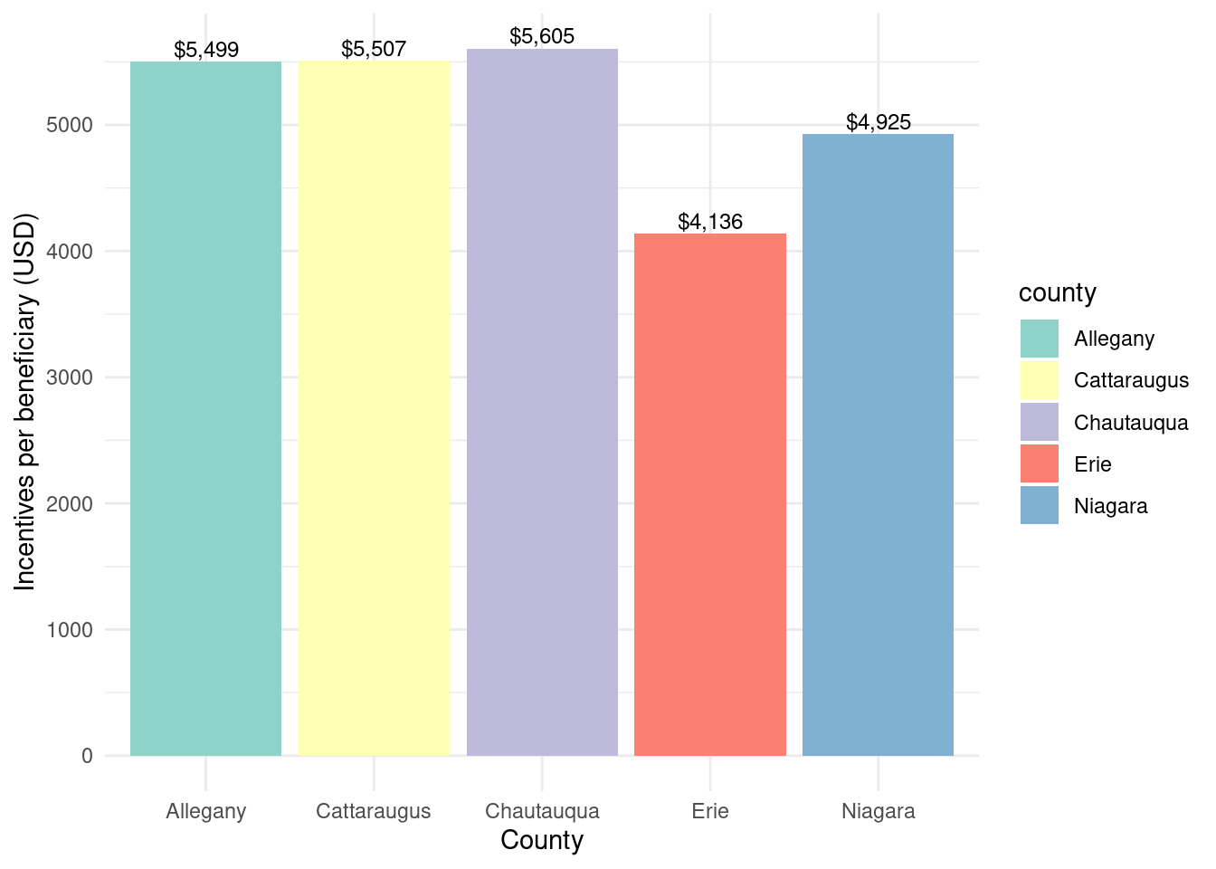
What percent of potential beneficiaries benefitted (by county)?

In [108]:

county_totalhh_wny <- zcta_hhlmi_wny |> 
  summarise(
    total_households = sum(total_households, na.rm = TRUE),
    .by = county
  )

county_totalstats_nysun_res_wny <- county_projectstats_nysun_resi_wny |> 
  inner_join(county_totalhh_wny, 
    by = join_by(county),
    relationship = "one-to-one",
    unmatched = "error"
  ) |>
  mutate(
    beneficiary_hh_pct = total_projects / total_households,
    incentives_per_beneficiary = total_incentives / total_projects,
    energycap_per_beneficiary = total_energy_capacity / total_projects,
    energygen_per_beneficiary = total_energy_generation / total_projects,
    total_private_investment = total_project_cost - total_incentives,
  )

In [109]:

In [110]:

county_totalstats_nysun_res_wny |>
  select(c(county, beneficiary_hh_pct, incentives_per_beneficiary)) |>
  mutate(across(c("beneficiary_hh_pct"), scales::label_percent(accuracy = 0.01))) |>
  mutate(across(where(is.numeric), scales::label_comma(accuracy = 1))) |>
  mutate(across(c("incentives_per_beneficiary"), function(x) paste0("$", as.character(x)))) |>
  knitr::kable(col.names = c("County",
                           "Recipients percentage",
                           "Incentives per beneficiary"))

NY-Sun Residential by beneficiary by county

County	Recipients percentage	Incentives per beneficiary
Allegany	0.82%	$5,499
Erie	0.78%	$4,136
Niagara	0.87%	$4,925
Cattaraugus	0.75%	$5,507
Chautauqua	0.72%	$5,605

In descending order the pct beneficiaries in each county that beneffited:

1 Niagara 0.869 2 Allegany 0.821 3 Erie 0.778 4 Cattaraugus 0.748 5 Chautauqua 0.723

Geography

Answers are coming from the county_totalstats_nysun_res_wny data frame created above:

Where are the potential beneficiaries?

By county? In desc order:

1 Erie 405436 2 Niagara 89556 3 Chautauqua 51886 4 Cattaraugus 29409 5 Allegany 16204

Where did this money go? In desc order here is where the incentives went by county:

1 Erie 13052190. 2 Niagara 3831428. 3 Chautauqua 2101823 4 Cattaraugus 1211624. 5 Allegany 731419.

Money over beneficiaries? In desc order by county:

1 Chautauqua 5605. 2 Cattaraugus 5507. 3 Allegany 5499. 4 Niagara 4925. 5 Erie 4136.

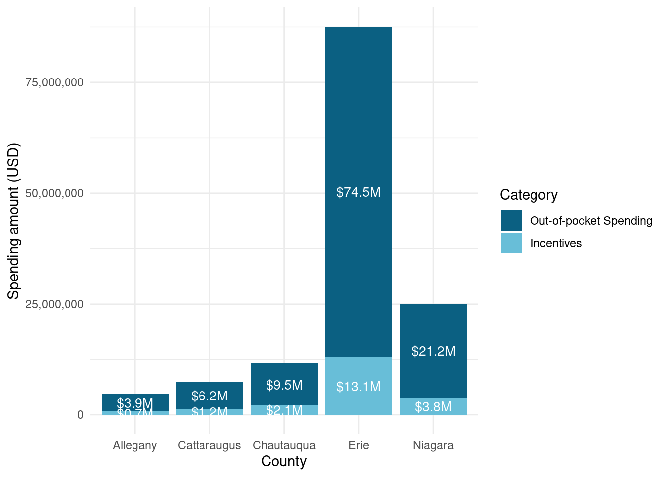
Some takeaways are: Erie once again has the highest # of potencial beneficiaries (probably due to its sheer size) and it also has the highest amount of incentives. Niagara comes 2nd in both again probably due to size/population.

When we look at incentives per beneficiary, the rural counties clearly recieve more money per person. Chataqua county is in the lead, followed by Cattaraugus and Allegany respectively. Erie County, despite getting most of the funding, has the lowest incentives per beneficiary. Is this because projects are more expensive in rural areas? Or was there just more of a focus there?

In [111]:

county_totalstats_nysun_res_wny_long <- county_totalstats_nysun_res_wny |>
  pivot_longer(
    cols = c(total_projects, total_incentives, total_private_investment, incentives_per_beneficiary),
    names_to = "category",
    values_to = "value"
  ) |>
  mutate(category = factor(category, 
                           levels = c("total_projects", 
                                      "total_private_investment",
                                      "total_incentives", 
                                      "incentives_per_beneficiary")))

Adding more readable labels for the graph!

In [112]:

labels <- as_labeller(c(
  "total_projects" = "Total Projects",
  "total_incentives" = "Total Incentives",
  "total_private_investment" = "Total Out-of-pocket",
  "incentives_per_beneficiary" = "Incentives per Beneficiary"
))

In [113]:

county_totalstats_nysun_res_wny_long |>
  filter(category %in% c("total_incentives", "total_private_investment")) |>
  ggplot(aes(x = county, y = value, fill = category)) +
  geom_bar(stat = "identity") +
  geom_text(
    aes(label = paste0("$", scales::comma(value/1000000, accuracy = 0.1), "M")), 
    position = position_stack(vjust = 0.5), 
    color = "white", 
    size = 3.5
  ) +
  scale_fill_manual(
    values = c(
      "total_incentives" = sky, 
      "total_private_investment" = midnight_lighter
    ),
    labels = c(
      "total_incentives" = "Incentives", 
      "total_private_investment" = "Out-of-pocket Spending"
    )
  ) +
  scale_y_continuous(labels = scales::comma) + 
  labs(
    x = "County",
    y = "Spending amount (USD)",
    fill = "Category"
  ) +
  theme_minimal()

graph showing projects, incentives, and incentives per beneficiary:

In [114]:

# Graphs not intuitive
county_totalstats_nysun_res_wny_long |> 
  ggplot(aes(x = county, y = value, fill = county)) +
  geom_bar(stat = "identity") +
  facet_wrap(~category, scales = "free_y", labeller = labels) +
  labs(title = "NY Sun Residential Projects, Incentives, and Incentives per Beneficiary 
        across Counties",
        x = "County",
        y = "Value") +
  theme_minimal() +
  scale_fill_brewer(palette = "Set3") + 
  scale_y_continuous(labels = scales::comma) + 
  theme(axis.text.x = element_text(angle = 45, hjust = 1), 
        strip.text.x = element_text(size = 7))

In [115]:

county_totalstats_nysun_res_wny |>
  ggplot(aes(x = county, y = incentives_per_beneficiary, fill = county)) +
  geom_bar(stat = "identity") +
  theme_minimal() +
  labs(x = "County",
      y = "Incentives per beneficiary (USD)") +
  geom_text(aes(label = paste0("$", scales::comma(incentives_per_beneficiary, accuracy = 1))),
          vjust = -0.3,
          color = "black",
          position = position_dodge(width = 0.9),
          size = 3.2) +
  scale_fill_brewer(palette = "Set3") +
  scale_y_continuous(breaks = seq(0, 10000, 1000))

Total incentives per beneficiary by county for NY-Sun Residential program

In [116]:

county_totalstats_nysun_res_wny |>
  ggplot(aes(x = county, y = energycap_per_beneficiary, fill = county)) +
  geom_bar(stat = "identity") +
  theme_minimal() +
  labs(x = "County",
      y = "Energy capacity per beneficiary (kW)") +
  geom_text(aes(label = scales::comma(energycap_per_beneficiary, accuracy = 0.01)),
          vjust = -0.3,
          color = "black",
          position = position_dodge(width = 0.9),
          size = 3.2) +
  scale_fill_brewer(palette = "Set3")

Energy capacity per installed system by county for NY-Sun Residential program

In [117]:

county_totalstats_nysun_res_wny |>
  ggplot(aes(x = county, y = energygen_per_beneficiary, fill = county)) +
  geom_bar(stat = "identity") +
  theme_minimal() +
  labs(x = "County",
      y = "Energy savings per beneficiary (kW)") +
  geom_text(aes(label = scales::comma(energygen_per_beneficiary, accuracy = 1)),
          vjust = -0.3,
          color = "black",
          position = position_dodge(width = 0.9),
          size = 3.2) +
  scale_fill_brewer(palette = "Set3")

Energy generated per installed PV system by county for Empower program

Race

What percent of beneficiaries are white vs. black vs. native vs. other?

In [118]:

county_totalstats_byrace_nysun_res_wny <- zcta_totalstats_nysun_res_wny |> 
  summarize(
    nysun_incentives_race = sum(nysun_incentives_race, 
      na.rm = TRUE),
    nysun_totalprojects_race = sum(nysun_totalprojects_race,
      na.rm = TRUE),
    nysun_totalhouseholds_race = sum(hh_by_race, na.rm = TRUE),
    .by = c(county, race)
  )

In [119]:

region_totalstats_byrace_nysun_res_wny <- county_totalstats_byrace_nysun_res_wny |>
  summarize(
    total_incentives_by_race = sum(nysun_incentives_race),
    total_race_hh = sum(nysun_totalhouseholds_race),
    .by = race) |>
  mutate(
    incentives_per_hh_by_race = total_incentives_by_race / total_race_hh
  )

In [120]:

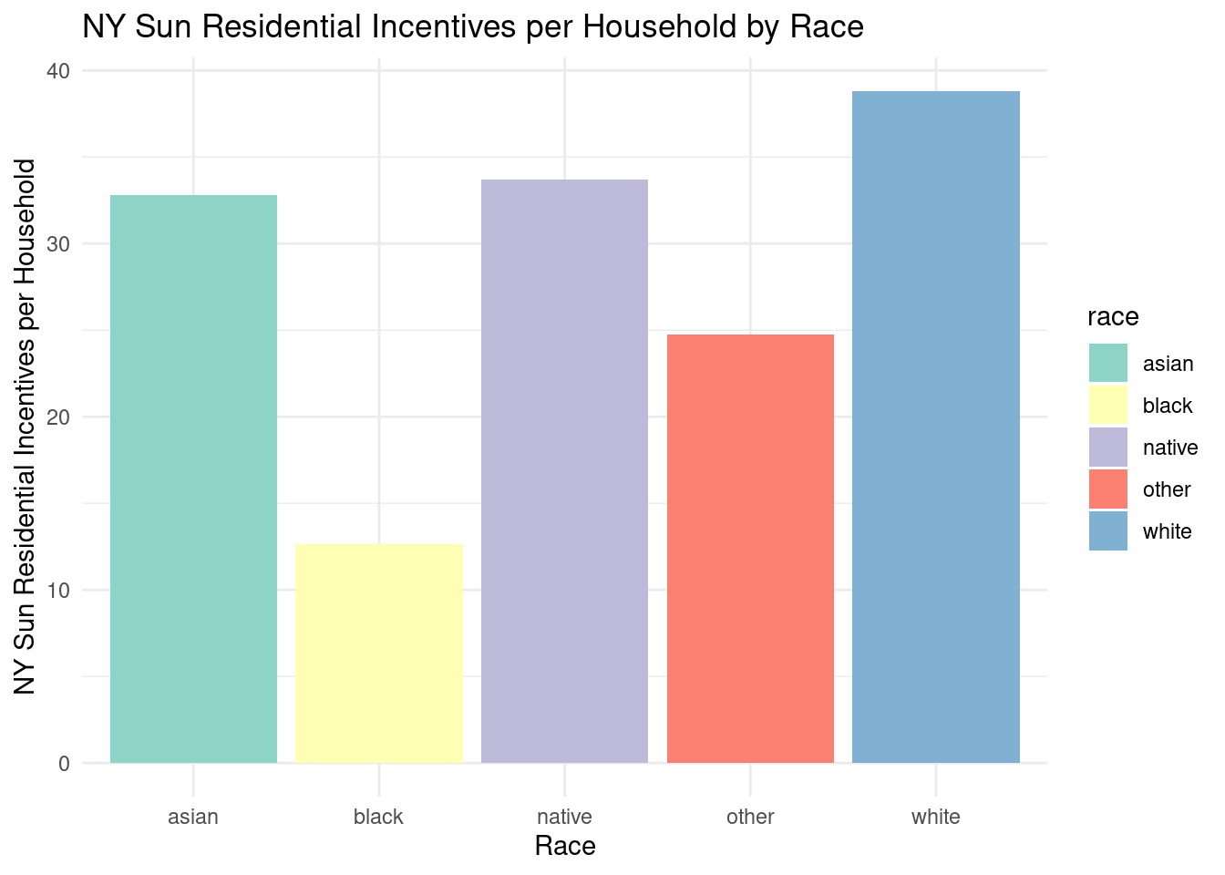
region_totalstats_byrace_nysun_res_wny |>
  ggplot(aes(x = race, y = incentives_per_hh_by_race, fill = race)) +
  geom_bar(stat = "identity") +
  labs(title = "NY Sun Residential Incentives per Household by Race",
       x = "Race",
       y = "NY Sun Residential Incentives per Household") +
  theme_minimal() +
  scale_fill_brewer(palette = "Set3")

In [121]:

zcta_totalhh_byrace_wny <- zctarace_hhlmi_wny |> 
  mutate(
    zcta_total_households = sum(total_households, na.rm = TRUE), 
    .by = zcta
  ) |>
  rename(hh_by_race = total_households) |>
  select(-c(li_households, 
            mi_households,
            lmi_households, 
            pct_li, pct_mi,   
            pct_lmi)
  )

zcta_totalstats_nysun_res_wny <- zip_projectstats_nysun_resi_wny |> 
  left_join(zcta_totalhh_byrace_wny, 
    by = join_by(zip == zcta)
  ) |> 
  filter(county != "NA")

zcta_totalstats_nysun_res_wny <- zcta_totalstats_nysun_res_wny |>
  mutate(
    racehh_zcta_percent = hh_by_race / zcta_total_households,
    nysun_incentives_race = racehh_zcta_percent * total_incentives,
    nysun_totalprojects_race = racehh_zcta_percent * total_projects,
    .by = c(zip,county)
  )

White households received the highest amount of NY Sun Residential incentive per household. Black households received the least amount of Residential incentive per household.

In [122]:

# not region level. double check to see what this does
region_pctstats_byrace_nysun_res_wny <- 
  county_totalstats_byrace_nysun_res_wny |>
    mutate(
      county_nysun_incentive_total = sum(nysun_incentives_race, 
        na.rm = TRUE),
      county_nysun_totalprojects_race_total = 
        sum(nysun_totalprojects_race, na.rm = TRUE),
      .by = county
    ) |> 
    mutate(
      nysun_incentive_race_county_pct = (nysun_incentives_race /
        county_nysun_incentive_total) * 100,
      nysun_totalprojects_race_pct = 
        (nysun_totalprojects_race / 
        county_nysun_totalprojects_race_total) * 100 
    )

In [123]:

region_totalstats_byrace_nysun_res_wny <- region_pctstats_byrace_nysun_res_wny |>
  summarise(total_projects = sum(nysun_totalprojects_race),
  total_hh = sum(nysun_totalhouseholds_race),
  total_incentives = sum(nysun_incentives_race),
  .by = race)

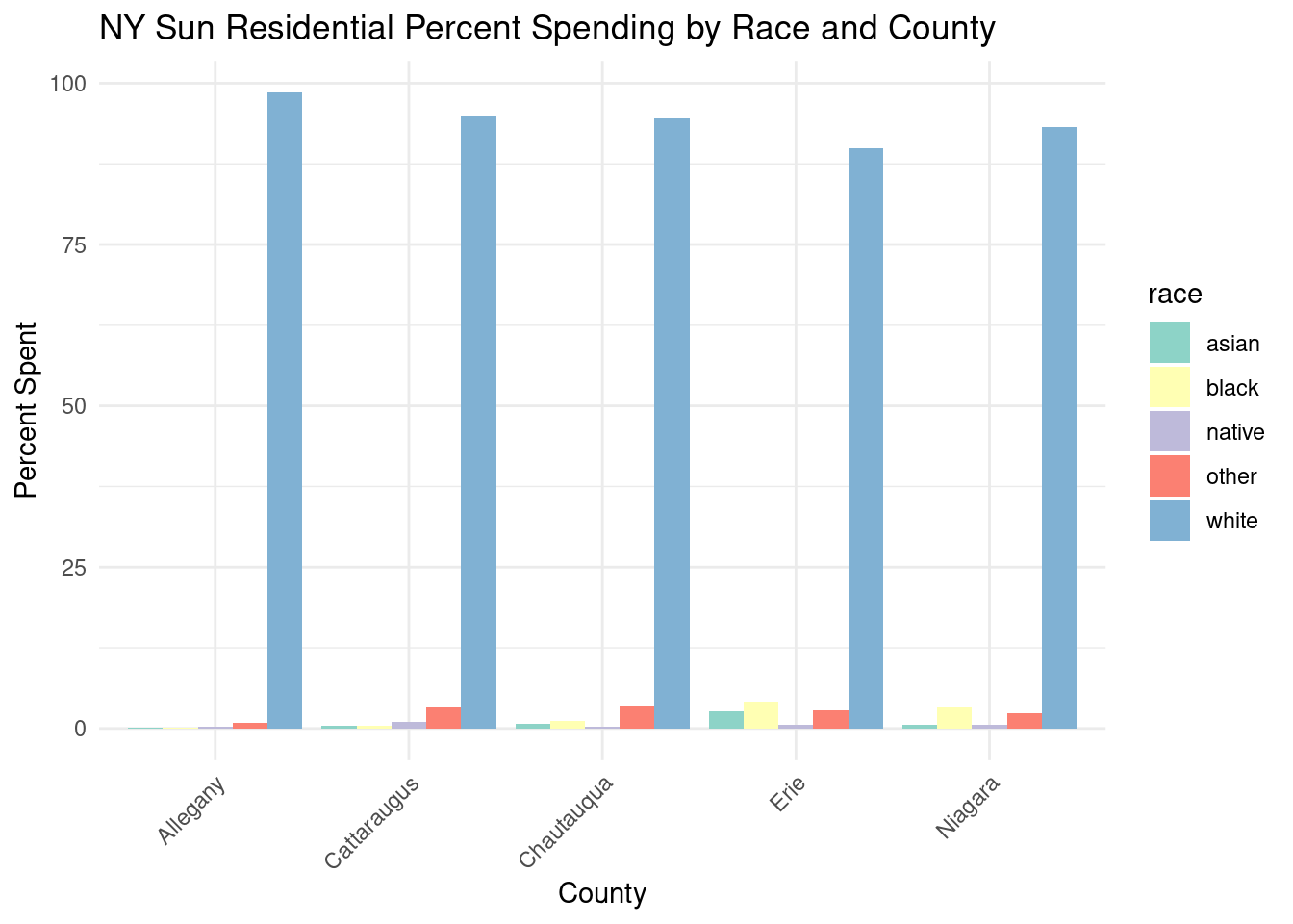
What percent of spending went to white vs. black vs. native vs. other?

By county the percent of spending went to:

1 Allegany white 98.5
2 Allegany black 0.170 3 Allegany native 0.330 4 Allegany asian 0.147 5 Allegany other 0.813

6 Erie white 89.9
7 Erie black 4.16 8 Erie native 0.536 9 Erie asian 2.62 10 Erie other 2.80

11 Cattaraugus white 94.9
12 Cattaraugus black 0.454 13 Cattaraugus native 0.999 14 Cattaraugus asian 0.360 15 Cattaraugus other 3.32

16 Niagara white 93.2
17 Niagara black 3.22 18 Niagara native 0.559 19 Niagara asian 0.583 20 Niagara other 2.41

21 Chautauqua white 94.5
22 Chautauqua black 1.12 23 Chautauqua native 0.335 24 Chautauqua asian 0.688 25 Chautauqua other 3.36

Graph showing the info above:

In [124]:

region_pctstats_byrace_nysun_res_wny |> 
ggplot(aes(x = county, y = nysun_incentive_race_county_pct, fill = race)) +
  geom_bar(stat = "identity", position = "dodge") +
  labs(title = "NY Sun Residential Percent Spending by Race and County",
       x = "County", y = "Percent Spent") +
  theme_minimal() +
  scale_fill_brewer(palette = "Set3") +
  theme(axis.text.x = element_text(angle = 45, hjust = 1))

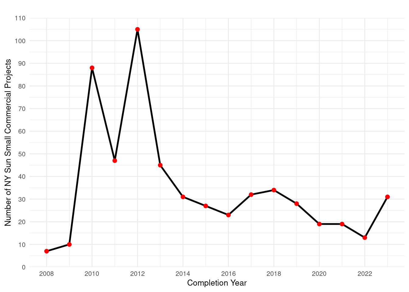
NY Sun Small Commercial

The df region_projectstats_nysun_scom_wny was created to show the overall number of projects, incentives, energy capacity, and energy generation in all of WNY.

In [125]:

region_projectstats_nysun_scom_wny <- county_projectstats_nysun_smallcomm_wny |> 
  summarize_if(is.numeric, sum, na.rm=TRUE)

In [126]:

region_totalstats_byrace_nysun_res_wny |>
  mutate(hh_pct = (total_hh / sum(total_hh)) * 100) |>
  mutate(hh_pct = as.numeric(format(round(hh_pct, 2), nsmall = 2))) |>
  ggplot(aes(y = hh_pct, x = race, fill = race)) +
  labs(y = "Percentage of total HH population (%)",
  x = "Race") +
  geom_bar(stat = "identity") +
  geom_text(aes(label = paste0(hh_pct, "%")), 
          vjust = -0.5, 
          color = "black", 
          size = 3.5) +
  theme_minimal()

In [127]:

region_totalstats_byrace_nysun_res_wny |>
  mutate(beneficiary_pct = (total_projects / sum(total_projects)) * 100) |>
  mutate(beneficiary_pct = as.numeric(format(round(beneficiary_pct, 2), nsmall = 2))) |>
  ggplot(aes(y = beneficiary_pct, x = race, fill = race)) +
  labs(y = "Percentage of household beneficiary (%)",
  x = "Race") +
  geom_bar(stat = "identity") +
  geom_text(aes(label = paste0(beneficiary_pct, "%")), 
          vjust = -0.5, 
          color = "black", 
          size = 3.5) +
  theme_minimal()

Racial makeup of NY-Sun Residential program’s beneficiary households in WNY

Big picture

Let’s drill in on the years 2008-2023.

In [128]:

projects_nysun_smallcomm_wny_08_23 <- projects_nysun_smallcomm |>
  filter(county %in% wny_counties) |> 
  mutate(completion_year = year(project_completion_date)) |>
1  filter(!is.na(completion_year)) |>
2  filter(completion_year > 2007 & completion_year < 2024)

1: Some of the projects have not yet been completed which is why those have been filtered out.
2: Earlier years have also been filtered out because few projects were completed during that time. We also filtered out 2024 since the year is not over.

How much money was spent overall in WNY?

In [129]:

smallcomm_wny_08_23_total_incentives <- projects_nysun_smallcomm_wny_08_23 |> summarize(sum(incentives, na.rm = TRUE))

smallcomm_wny_08_23_total_incentives

# A tibble: 1 × 1
  `sum(incentives, na.rm = TRUE)`
                            <dbl>
1                       37923056.

Answer: $37,923,056

On how many projects?

In [130]:

smallcomm_wny_08_23_total_projects <- projects_nysun_smallcomm_wny_08_23 |> summarize(n())

smallcomm_wny_08_23_total_projects

# A tibble: 1 × 1
  `n()`
  <int>
1   559

Answer: 559

Average spending per project?

In [131]:

smallcomm_wny_08_23_total_incentives / smallcomm_wny_08_23_total_projects

  sum(incentives, na.rm = TRUE)
1                      67840.89

Answer: $67,840.89

How much private investment did that catalyze?

In [132]:

projects_nysun_smallcomm_wny_08_23 |> 
  summarize(sum(project_cost - incentives, na.rm = TRUE))

# A tibble: 1 × 1
  `sum(project_cost - incentives, na.rm = TRUE)`
                                           <dbl>
1                                      81316349.

Answer: $81,316,349

How much data total project cost data is missing?

In [133]:

projects_nysun_smallcomm_wny_08_23 |> 
  mutate(
    project_cost_zero = project_cost == 0,
    project_cost_missing = is.na(project_cost)
  ) |> 
  summarize(
    sum(project_cost_missing) / n(),
    sum(project_cost_zero) / n(),
  )

# A tibble: 1 × 2
  `sum(project_cost_missing)/n()` `sum(project_cost_zero)/n()`
                            <dbl>                        <dbl>
1                               0                       0.0161

Very little, so we use this figure.

How much solar capacity did that add?

In [134]:

projects_nysun_smallcomm_wny_08_23 |> 
  summarize(sum(energy_capacity, na.rm = TRUE))

# A tibble: 1 × 1
  `sum(energy_capacity, na.rm = TRUE)`
                                 <dbl>
1                               38364.

38,364 kW, or 38 mW.

What is the average capacity per project?

In [135]:

projects_nysun_smallcomm_wny_08_23 |> 
  summarize(sum(energy_capacity, na.rm = TRUE) / n())

# A tibble: 1 × 1
  `sum(energy_capacity, na.rm = TRUE)/n()`
                                     <dbl>
1                                     68.6

68.6 kW.

How much of the solar capacity data is missing?

In [136]:

projects_nysun_smallcomm_wny_08_23 |> 
  mutate(
    energy_capacity_zero = energy_capacity == 0,
    energy_capacity_missing = is.na(energy_capacity)
  ) |> 
  summarize(
    sum(energy_capacity_missing) / n(),
    sum(energy_capacity_zero) / n(),
  )

# A tibble: 1 × 2
  `sum(energy_capacity_missing)/n()` `sum(energy_capacity_zero)/n()`
                               <dbl>                           <dbl>
1                                  0                         0.00179

Almost none, so we can use the data.

Projects completed over time?

In [137]:

region_projectcountbyyear_nysun_res_wny <- projects_nysun_smallcomm_wny_08_23 |>
  summarise(
    project_count_by_year = sum(project_count = n()),
    .by = completion_year
  )

The scatterplot below shows the projects completed over time:

In [138]:

region_projectcountbyyear_nysun_res_wny |> 
  ggplot(aes(x = completion_year, y = project_count_by_year, group = 1)) +
    geom_line(color = "black", linewidth = 1) +
    geom_point(color = "red", size = 2) +
    labs(
      title = "",
      x = "Completion Year",
      y = "Number of NY Sun Small Commercial Projects",
    )  +
    theme_minimal() +
    scale_x_continuous(breaks = seq(2004, 2023, 2)) +
    scale_y_continuous(breaks = seq(0, 110, 10),  limit = c(0, 110), expand = c(0, NA)) +
    theme(
      plot.title = element_text(size = 12, face = "bold"),
      axis.title = element_text(size = 10),
      axis.text = element_text(size = 8),
      plot.caption = element_text(size = 8, hjust = 1)
  )

Completed NY Sun small commercial projects by year

There is less of a dip for 2020 than for other programs.

How much money was spent county? In desc order:

1 Erie 32,906,643. 2 Niagara 5,029,240 3 Chautauqua 2,273,620. 4 Cattaraugus 1,230,090. 5 Allegany 237,538

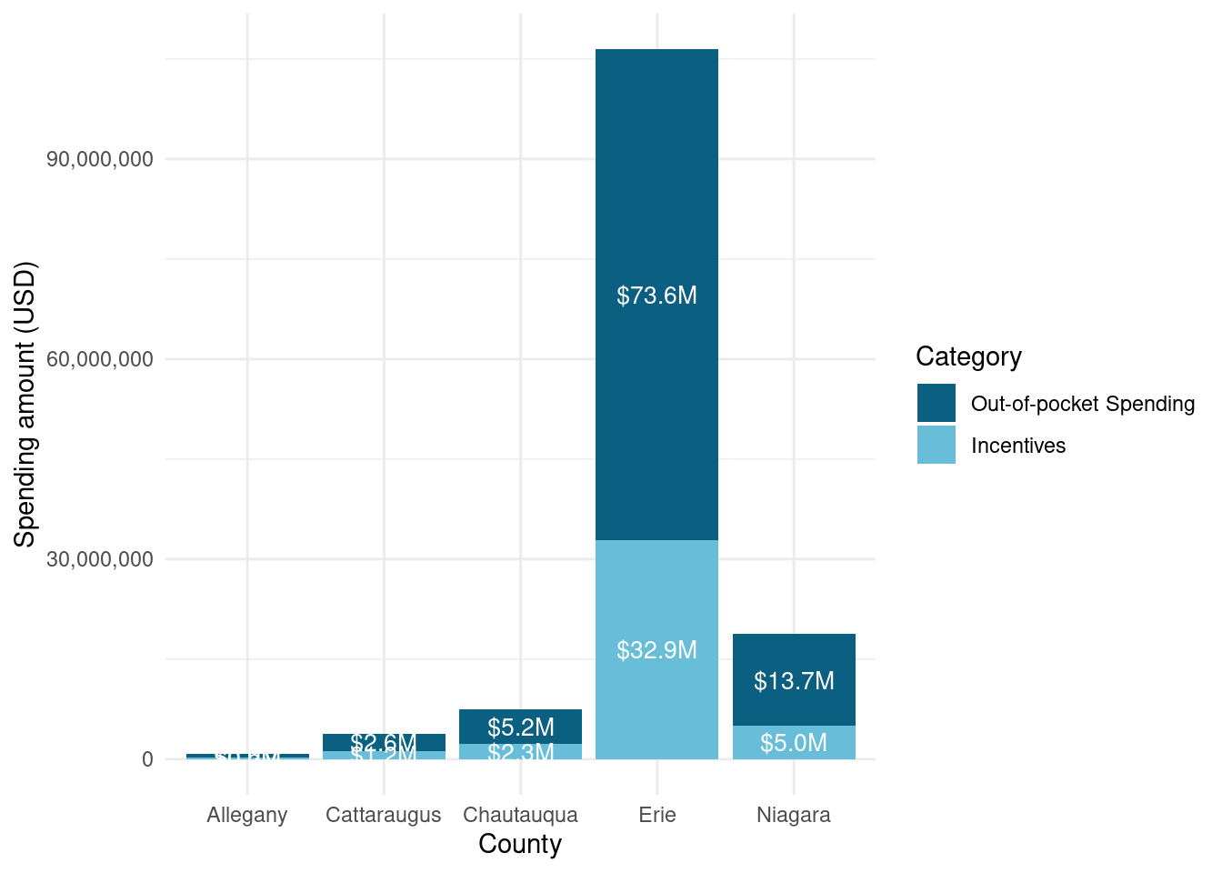
Erie has by far the most money spent for small commercial projects, more than would be expected even given its much larger size than the other counties by population.

What percent of potential beneficiaries benefitted? non applicable to commercial projects.

How much energy capacity? (kw)

By county in desc order:

1 Erie 35,742. 2 Niagara 7,005. 3 Chautauqua 2,844. 4 Cattaraugus 1,542. 5 Allegany 343.

Erie has the highest energy capacity, and about 5x the energy capacity of the next highest county (Niagara).

Graph showing spending and energy capacity:

In [139]:

county_projectstats_nysun_smallcomm_wny_long <- county_projectstats_nysun_smallcomm_wny |>
  mutate(
    total_private_investment = total_project_cost - total_incentives
  ) |>
  pivot_longer(
    cols = c(total_incentives, total_private_investment, total_energy_capacity),
    names_to = "category",
    values_to = "value"
  ) |>
  mutate(category = factor(
    category, 
    levels = c("total_private_investment", "total_incentives", "total_energy_capacity")
  ))

In [140]:

labels_smallcomm <- as_labeller(c(
  "total_incentives" = "Total Incentives",
  "total_incentives" = "Total Out-of-pocket",
  "total_energy_capacity" = "Energy Capacity (kW)"
))

In [141]:

county_projectstats_nysun_smallcomm_wny_long |>
  filter(category %in% c("total_incentives", "total_private_investment")) |>
  ggplot(aes(x = county, y = value, fill = category)) +
  geom_bar(stat = "identity") +
  geom_text(
    aes(label = paste0("$", scales::comma(value/1000000, accuracy = 0.1), "M")), 
    position = position_stack(vjust = 0.5), 
    color = "white", 
    size = 3.5
  ) +
  scale_fill_manual(
    values = c(
      "total_incentives" = sky, 
      "total_private_investment" = midnight_lighter
    ),
    labels = c(
      "total_incentives" = "Incentives", 
      "total_private_investment" = "Out-of-pocket Spending"
    )
  ) +
  scale_y_continuous(labels = scales::comma) + 
  labs(
    x = "County",
    y = "Spending amount (USD)",
    fill = "Category"
  ) +
  theme_minimal()

In [142]:

county_totalstats_nysun_smallcomm_wny <- county_projectstats_nysun_smallcomm_wny |> 
  inner_join(county_totalhh_wny, 
    by = join_by(county),
    relationship = "one-to-one",
    unmatched = "error"
  ) |>
  mutate(
    beneficiary_hh_pct = total_projects / total_households,
    incentives_per_beneficiary = total_incentives / total_projects,
    energycap_per_beneficiary = total_energy_capacity / total_projects,
    energygen_per_beneficiary = total_energy_generation / total_projects,
    total_private_investment = total_project_cost - total_incentives,
  )

In [143]:

county_projectstats_nysun_smallcomm_wny_long |> 
  ggplot(aes(x = county, y = value, fill = county)) +
  geom_bar(stat = "identity") +
  facet_wrap(~category, scales = "free_y", labeller = labels_smallcomm) +
  labs(
    title = "NY Sun Small Commercial Incentives and Energy Capacity across Counties",
    x = "County",
    y = "Value"
  ) +
  theme_minimal() +
  scale_fill_brewer(palette = "Set3") +
  scale_y_continuous(labels = scales::comma) +
  theme(
    axis.text.x = element_text(angle = 45, hjust = 1),
    strip.text.x = element_text(size = 7)
  )

Geography

Where are the potential beneficiaries? unsure how to answer this for commercial projects. We can simply show where the projects are at the most?

Where did this money go? same as “How much money was spent county?” probably

Money over projects? In desc order:

1 Niagara 73,959. 2 Erie 69,132. 3 Cattaraugus 51,254. 4 Chautauqua 41,339. 5 Allegany 26,393.

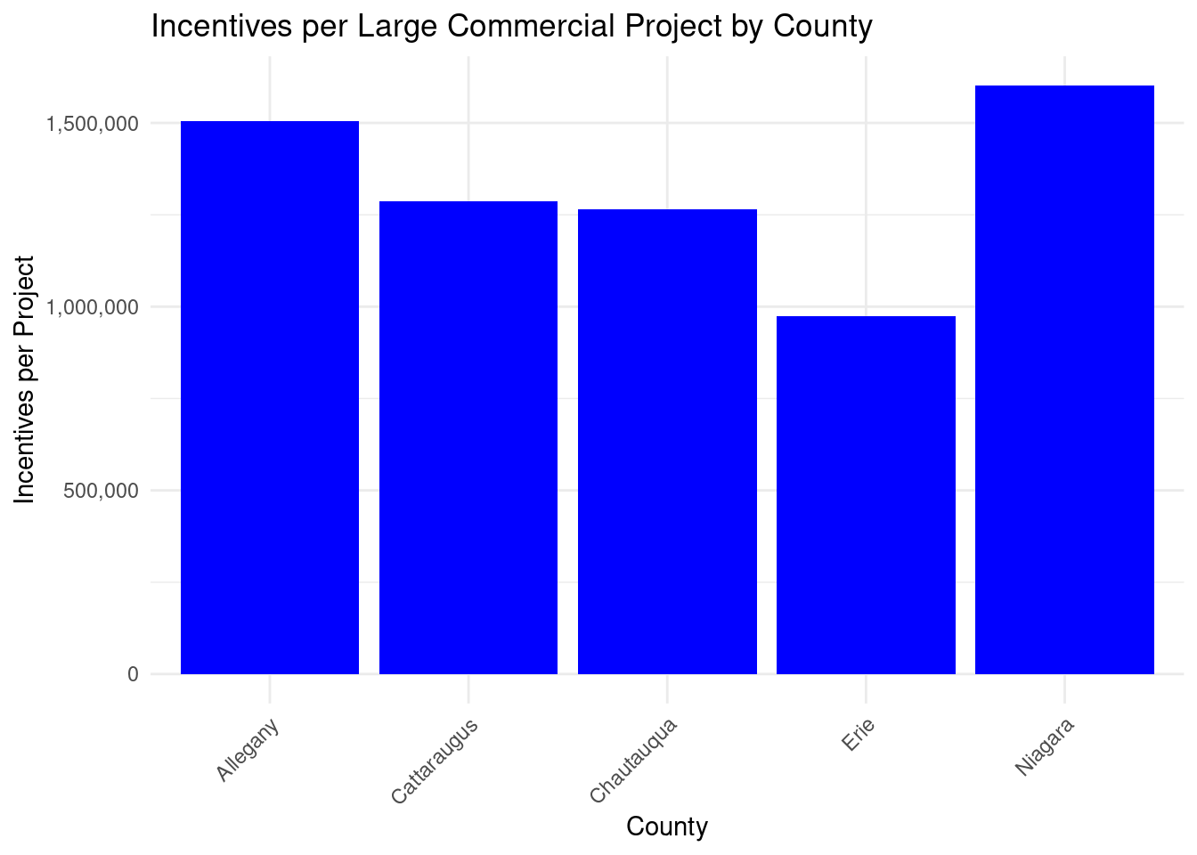
Projects were most expensive in Niagara and Erie counties, with much less spent per project in other counties, particularly in Allegany. It seems that more rural counties had less expensive projects.

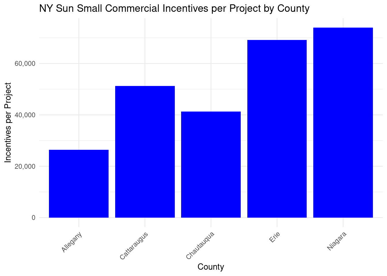
Graph showing the above:

In [144]:

county_projectstats_nysun_smallcomm_wny |>
  mutate(
    incentives_per_project = total_incentives / total_projects,
  ) |>
  distinct(county, incentives_per_project) |>
  ggplot(aes(x = county, y = incentives_per_project)) +
  geom_bar(stat = "identity", fill = "blue") +
  labs(
    title = "NY Sun Small Commercial Incentives per Project by County",
    x = "County",
    y = "Incentives per Project"
  ) +
  theme_minimal() +
  scale_y_continuous(labels = scales::comma) +  
  theme(axis.text.x = element_text(angle = 45, hjust = 1))

In [145]:

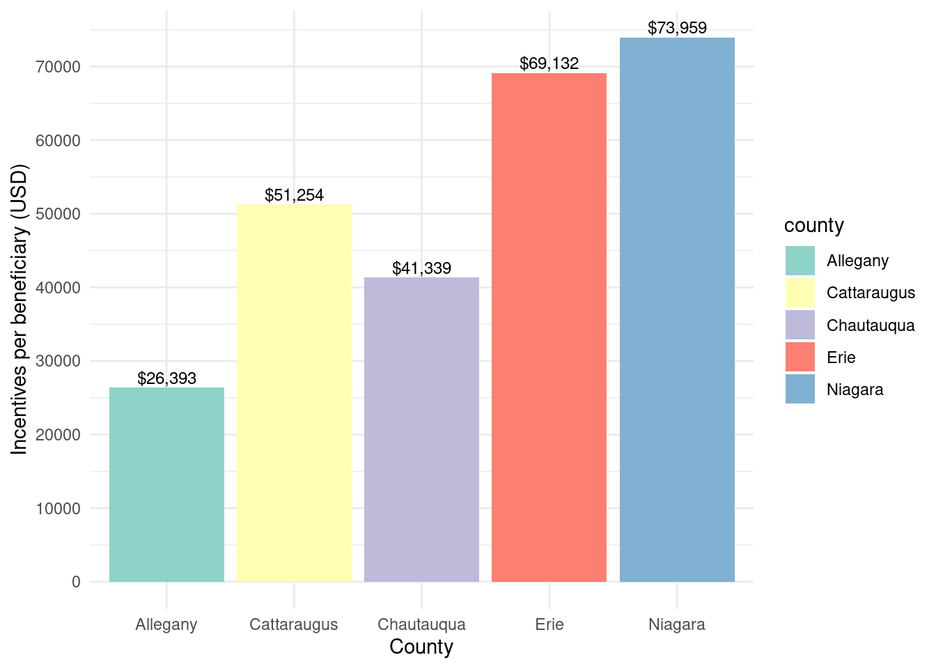
county_totalstats_nysun_smallcomm_wny |>
  ggplot(aes(x = county, y = incentives_per_beneficiary, fill = county)) +
  geom_bar(stat = "identity") +
  theme_minimal() +
  labs(x = "County",
      y = "Incentives per beneficiary (USD)") +
  geom_text(aes(label = paste0("$", scales::comma(incentives_per_beneficiary, accuracy = 1))),
          vjust = -0.3,
          color = "black",
          position = position_dodge(width = 0.9),
          size = 3.2) +
  scale_fill_brewer(palette = "Set3") +
  scale_y_continuous(breaks = seq(0, 100000, 10000))

Total incentives per beneficiary by county for NY-Sun Small Commercial program

In [146]:

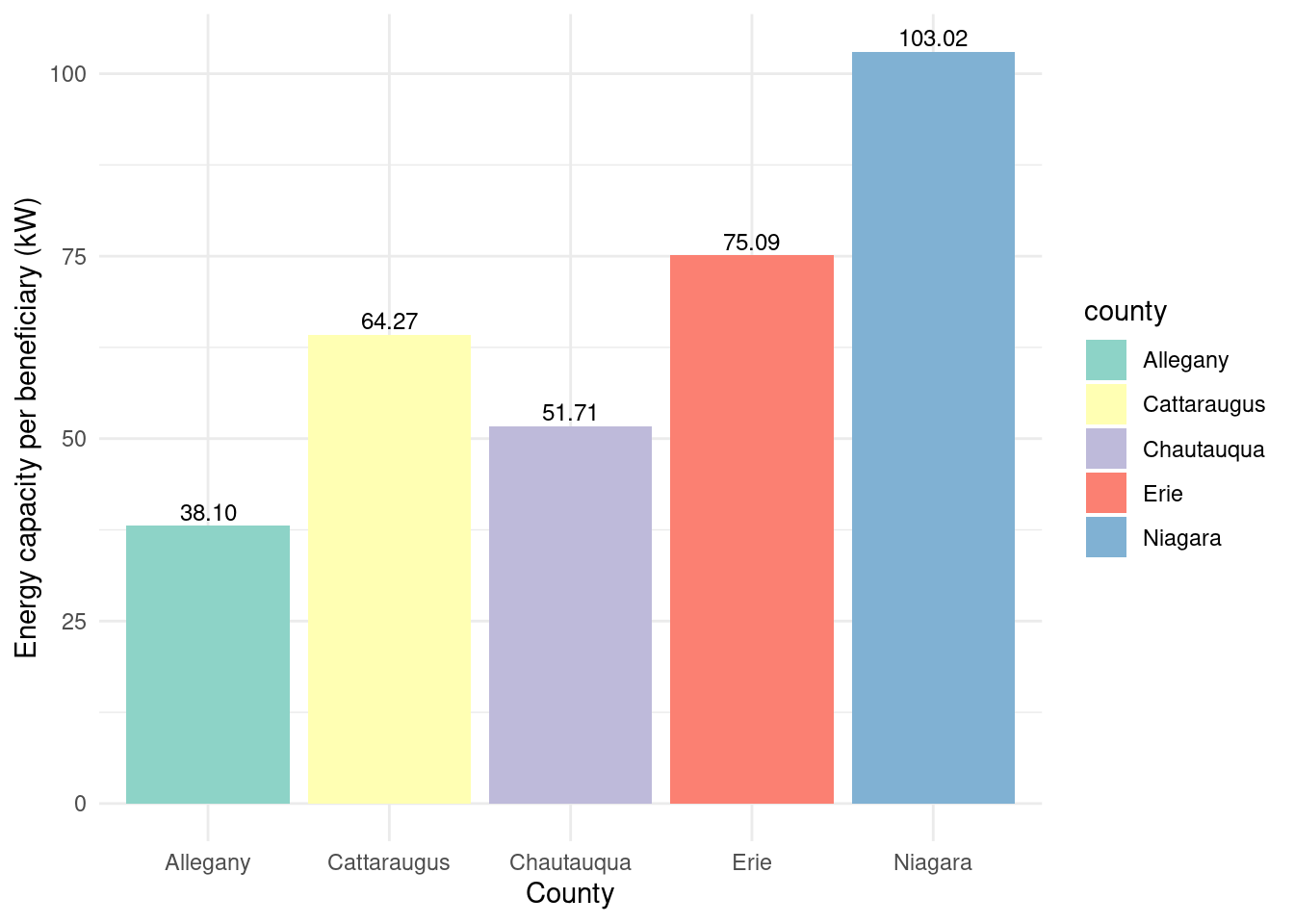
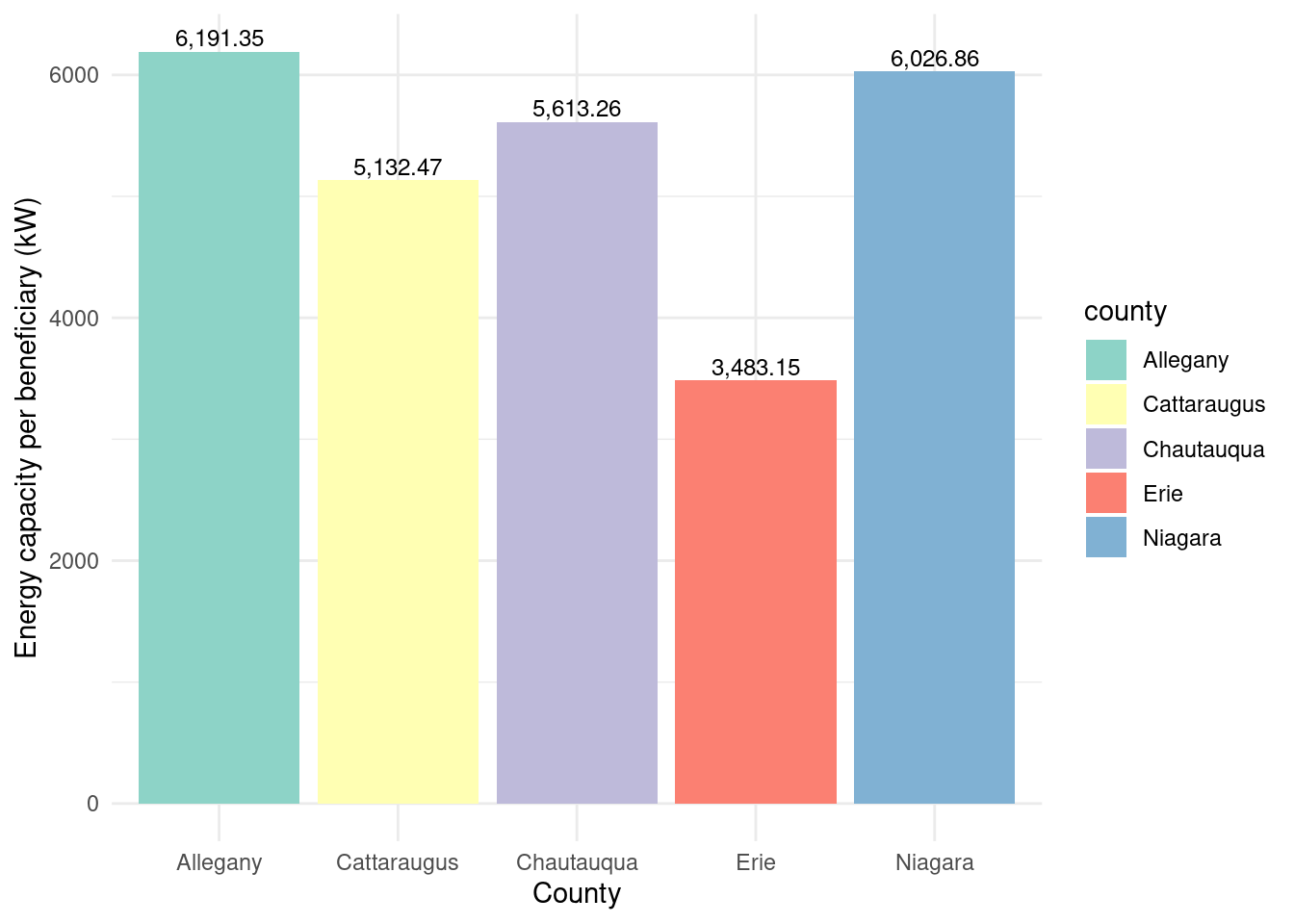
county_totalstats_nysun_smallcomm_wny |>
  ggplot(aes(x = county, y = energycap_per_beneficiary, fill = county)) +
  geom_bar(stat = "identity") +
  theme_minimal() +
  labs(x = "County",
      y = "Energy capacity per beneficiary (kW)") +
  geom_text(aes(label = scales::comma(energycap_per_beneficiary, accuracy = 0.01)),
          vjust = -0.3,
          color = "black",
          position = position_dodge(width = 0.9),
          size = 3.2) +
  scale_fill_brewer(palette = "Set3")

Energy capacity per installed system by county for NY-Sun Small Commercial program

NY Sun Large Commercial

Big picture

Let’s drill in on the years 2008-2023.

In [147]:

projects_nysun_largecomm_wny_08_23 <- projects_nysun_largecomm |>
  filter(county %in% wny_counties) |> 
  mutate(completion_year = year(project_completion_date)) |>
1  filter(!is.na(completion_year)) |>
2  filter(completion_year > 2007 & completion_year < 2024)

1: Some of the projects have not yet been completed which is why those have been filtered out.
2: Earlier years have also been filtered out because few projects were completed during that time. We also filtered out 2024 since the year is not over.

How much money was spent overall in WNY?

In [148]:

largecomm_wny_08_23_total_incentives <- projects_nysun_largecomm_wny_08_23 |> 
  summarize(sum(incentives, na.rm = TRUE))

largecomm_wny_08_23_total_incentives

# A tibble: 1 × 1
  `sum(incentives, na.rm = TRUE)`
                            <dbl>
1                       65802249.

Answer: $65,802,249

On how many projects?

In [149]:

largecomm_wny_08_23_total_projects <- projects_nysun_largecomm_wny_08_23 |> summarize(n())

largecomm_wny_08_23_total_projects

# A tibble: 1 × 1
  `n()`
  <int>
1    64

Answer: 64

Average spending per project?

In [150]:

largecomm_wny_08_23_total_incentives / largecomm_wny_08_23_total_projects

  sum(incentives, na.rm = TRUE)
1                       1028160

Answer: $1,028,160

How much private investment did that catalyze?

In [151]:

projects_nysun_largecomm_wny_08_23 |> 
  summarize(sum(project_cost - incentives, na.rm = TRUE))

# A tibble: 1 × 1
  `sum(project_cost - incentives, na.rm = TRUE)`
                                           <dbl>
1                                     283664619.

Answer: $283,664,619

How much data total project cost data is missing?

In [152]:

projects_nysun_largecomm_wny_08_23 |> 
  mutate(
    project_cost_zero = project_cost == 0,
    project_cost_missing = is.na(project_cost)
  ) |> 
  summarize(
    sum(project_cost_missing) / n(),
    sum(project_cost_zero) / n(),
  )

# A tibble: 1 × 2
  `sum(project_cost_missing)/n()` `sum(project_cost_zero)/n()`
                            <dbl>                        <dbl>
1                               0                            0

None, so we use this figure.

How much solar capacity did that add?

In [153]:

projects_nysun_largecomm_wny_08_23 |> 
  summarize(sum(energy_capacity, na.rm = TRUE))

# A tibble: 1 × 1
  `sum(energy_capacity, na.rm = TRUE)`
                                 <dbl>
1                              240655.

240,655 kW, or 240 MW.

What is the average capacity per project?

In [154]:

projects_nysun_largecomm_wny_08_23 |> 
  summarize(sum(energy_capacity, na.rm = TRUE) / n())

# A tibble: 1 × 1
  `sum(energy_capacity, na.rm = TRUE)/n()`
                                     <dbl>
1                                    3760.

3760 kW, or 3.7 MW.

How much of the solar capacity data is missing?

In [155]:

projects_nysun_largecomm_wny_08_23 |> 
  mutate(
    energy_capacity_zero = energy_capacity == 0,
    energy_capacity_missing = is.na(energy_capacity)
  ) |> 
  summarize(
    sum(energy_capacity_missing) / n(),
    sum(energy_capacity_zero) / n(),
  )

# A tibble: 1 × 2
  `sum(energy_capacity_missing)/n()` `sum(energy_capacity_zero)/n()`
                               <dbl>                           <dbl>
1                                  0                               0

None, so we can use the data.

Projects completed over time?

In [156]:

region_projectcountbyyear_nysun_res_wny <- projects_nysun_largecomm_wny_08_23 |>
  summarise(
    project_count_by_year = sum(project_count = n()),
    .by = completion_year
  )

The scatterplot below shows the projects completed over time:

In [157]:

region_projectcountbyyear_nysun_res_wny |> 
  ggplot(aes(x = completion_year, y = project_count_by_year, group = 1)) +
    geom_line(color = "black", linewidth = 1) +
    geom_point(color = "red", size = 2) +
    labs(
      title = "",
      x = "Completion Year",
      y = "# of Completed Projects",
    )  +
    theme_minimal() +
    scale_x_continuous(breaks = seq(2004, 2023, 2)) +
    scale_y_continuous(breaks = seq(0, 15, 2),  limit = c(0, 15), expand = c(0, NA)) +
    theme(
      plot.title = element_text(size = 12, face = "bold"),
      axis.title = element_text(size = 10),
      axis.text = element_text(size = 8),
      plot.caption = element_text(size = 8, hjust = 1)
  )

The scatterplot below shows the projects completed over time:

In [158]:

projects_nysun_large_yr <- projects_nysun_largecomm |>
  mutate(completion_year = year(project_completion_date)
  ) |>
1  filter(!is.na(completion_year)) |>
  summarise(
    project_count_by_year = sum(project_count = n()),
    .by = completion_year
  )

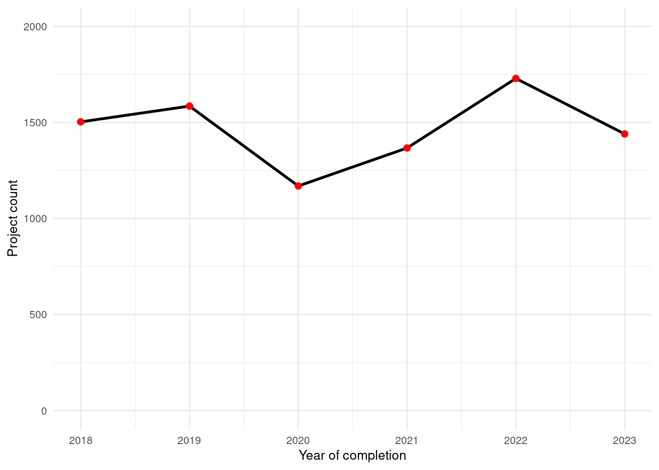
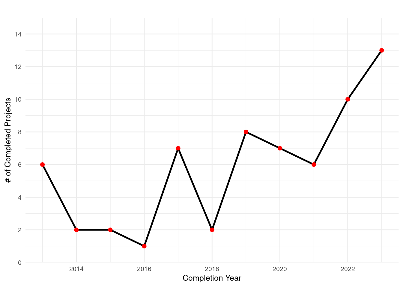
1: Some of the projects have not yet been completed which is why those have been filtered out.

In [159]:

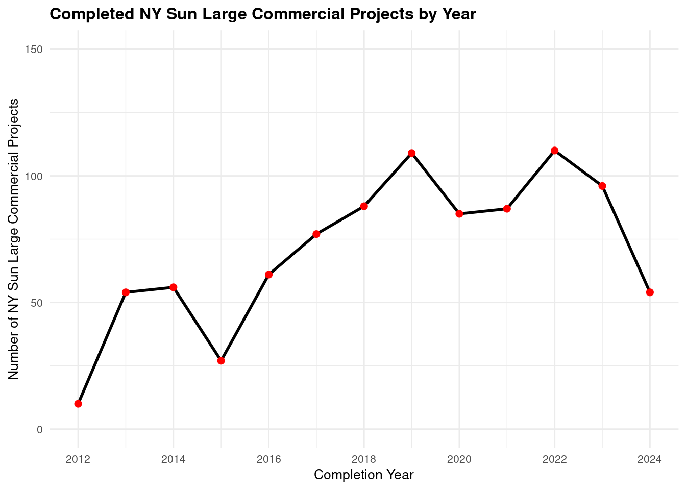
projects_nysun_large_yr |> 
  ggplot(aes(x = completion_year, y = project_count_by_year, group = 1)) +
  geom_line(color = "black", linewidth = 1) +
  geom_point(color = "red", size = 2) +
  labs(
    title = "Completed NY Sun Large Commercial Projects by Year",
    x = "Completion Year",
    y = "Number of NY Sun Large Commercial Projects"
  ) +
  scale_x_continuous(breaks = seq(min(projects_nysun_large_yr$completion_year), 
                                  max(projects_nysun_large_yr$completion_year), 
                                  by = 2)) + 
  scale_y_continuous(breaks = seq(0, 150, by = 50), limits = c(0, 150)) +  
  theme_minimal() +
  theme(
    plot.title = element_text(size = 12, face = "bold"),
    axis.title = element_text(size = 10),
    axis.text = element_text(size = 8),
    plot.caption = element_text(size = 8, hjust = 1)
  )

As with NY Sun small commercial, not much of a decrease in 2020, whereas Assisted and Empower had significant drops in number of projects per year in 2020. It could be that commercial projects did not experience a decrease in number during the pandemic, while household projects were more affected.

Money spent by county? in desc order:

1 Erie 47,674,765. 2 Chautauqua 45,555,346. 3 Niagara 36,828,770. 4 Cattaraugus 33,463,052. 5 Allegany 33,124,546.

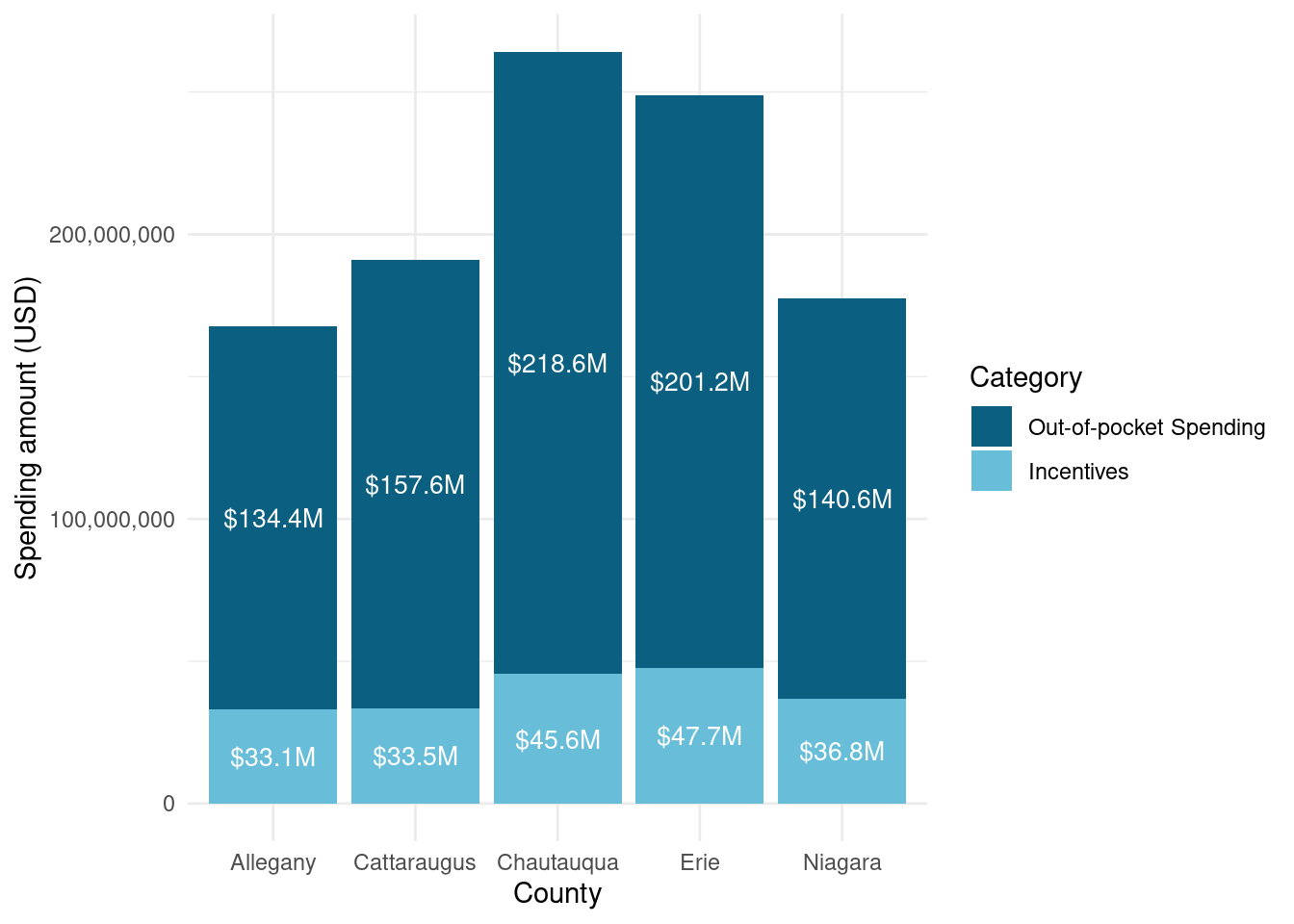
The range of incentives per county is fairly low. Erie and Chautauqua had similar amounts of spending per county, and Allegany had only about 30% less spending than Erie. This is surprising given how much bigger population is in Erie, however counties had small numbers of large commercial projects overall (for example, only 49 projects in Erie).

What percent of potential beneficiaries benefitted? Cannot be calculated for commercial projects as we have hh info only.

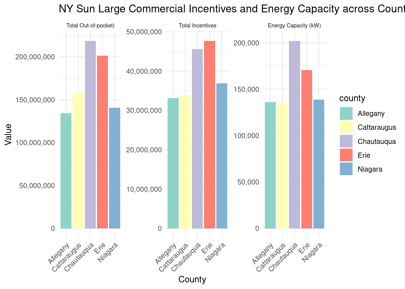
How much energy capacity? (kw) By county in desc order:

1 Chautauqua 202,077. 2 Erie 170,674. 3 Niagara 138,618. 4 Allegany 136,210. 5 Cattaraugus 133,444.

Projects in Chautauqua had larger energy capacity than other counties.

Graph showing spending and energy capacity:

In [160]:

county_projectstats_nysun_largecomm_wny_long <- county_projectstats_nysun_largecomm_wny |>
  mutate(
    total_private_investment = total_project_cost - total_incentives,
  ) |>
  pivot_longer(
    cols = c(total_private_investment, total_incentives, total_energy_capacity),
    names_to = "category",
    values_to = "value"
  ) |>
  mutate(category = factor(
    category, 
    levels = c("total_private_investment", "total_incentives", "total_energy_capacity")
  ))

In [161]:

labels_largecomm <- as_labeller(c(
  "total_incentives" = "Total Incentives",
  "total_private_investment" = "Total Out-of-pocket)",
  "total_energy_capacity" = "Energy Capacity (kW)"
))

In [162]:

county_projectstats_nysun_largecomm_wny_long |>
  filter(category %in% c("total_incentives", "total_private_investment")) |>
  ggplot(aes(x = county, y = value, fill = category)) +
  geom_bar(stat = "identity") +
  geom_text(
    aes(label = paste0("$", scales::comma(value/1000000, accuracy = 0.1), "M")), 
    position = position_stack(vjust = 0.5), 
    color = "white", 
    size = 3.5
  ) +
  scale_fill_manual(
    values = c(
      "total_incentives" = sky, 
      "total_private_investment" = midnight_lighter
    ),
    labels = c(
      "total_incentives" = "Incentives", 
      "total_private_investment" = "Out-of-pocket Spending"
    )
  ) +
  scale_y_continuous(labels = scales::comma) + 
  labs(
    x = "County",
    y = "Spending amount (USD)",
    fill = "Category"
  ) +
  theme_minimal()

In [163]:

county_projectstats_nysun_largecomm_wny_long |> 
  ggplot(aes(x = county, y = value, fill = county)) +
  geom_bar(stat = "identity") +
  facet_wrap(~category, scales = "free_y", labeller = labels_largecomm) +
  labs(
    title = "NY Sun Large Commercial Incentives and Energy Capacity across Counties",
    x = "County",
    y = "Value"
  ) +
  theme_minimal() +
  scale_fill_brewer(palette = "Set3") +
  scale_y_continuous(labels = scales::comma) +
  theme(
    axis.text.x = element_text(angle = 45, hjust = 1),
    strip.text.x = element_text(size = 7)
  )

While it could be reasonable to assume that more incentives/spending could lead to higher energy capacity, this does not seem to be the case particularly in Erie and Chatauqua. On the other hand, it seems like there might be some correlation in Allegany, Cattaraugus and Niagara.

Could it be that it is more expensive to build in some counties than others, and this is reflected in differing incentive amounts? Clearly there is some external influence affecting the relationship between incentives and energy capacity that we are unable to directly observe. ### Geography

Where are the potential beneficiaries?

By county?

Answering this as large commercial projects per county:

1 Erie 49 2 Chautauqua 36 3 Cattaraugus 26 4 Niagara 23 5 Allegany 22

Where did this money go? same as: “Money spent by county?” probably

Money over beneficiaries?

This has been calculated as incentives/projects:

1 Niagara 1,601,251. 2 Allegany 1,505,661. 3 Cattaraugus 1,287,040. 4 Chautauqua 1,265,426. 5 Erie 972,954.

It appears projects were more expensive in Niagara and Allegany counties.

Graph showing the above:

In [164]:

county_projectstats_nysun_largecomm_wny |>
  mutate(
    incentives_per_project = total_incentives / total_projects,
  ) |>
  distinct(county, incentives_per_project) |>
  ggplot(aes(x = county, y = incentives_per_project)) +
  geom_bar(stat = "identity", fill = "blue") +
  labs(
    title = "Incentives per Large Commercial Project by County",
    x = "County",
    y = "Incentives per Project"
  ) +
  theme_minimal() +
  scale_y_continuous(labels = scales::comma) +  
  theme(axis.text.x = element_text(angle = 45, hjust = 1))

In [165]:

county_totalstats_nysun_largecomm_wny <- county_projectstats_nysun_largecomm_wny |> 
  inner_join(county_totalhh_wny, 
    by = join_by(county),
    relationship = "one-to-one",
    unmatched = "error"
  ) |>
  mutate(
    beneficiary_hh_pct = total_projects / total_households,
    incentives_per_beneficiary = total_incentives / total_projects,
    energycap_per_beneficiary = total_energy_capacity / total_projects,
    energygen_per_beneficiary = total_energy_generation / total_projects,
    total_private_investment = total_project_cost - total_incentives,
  )

In [166]:

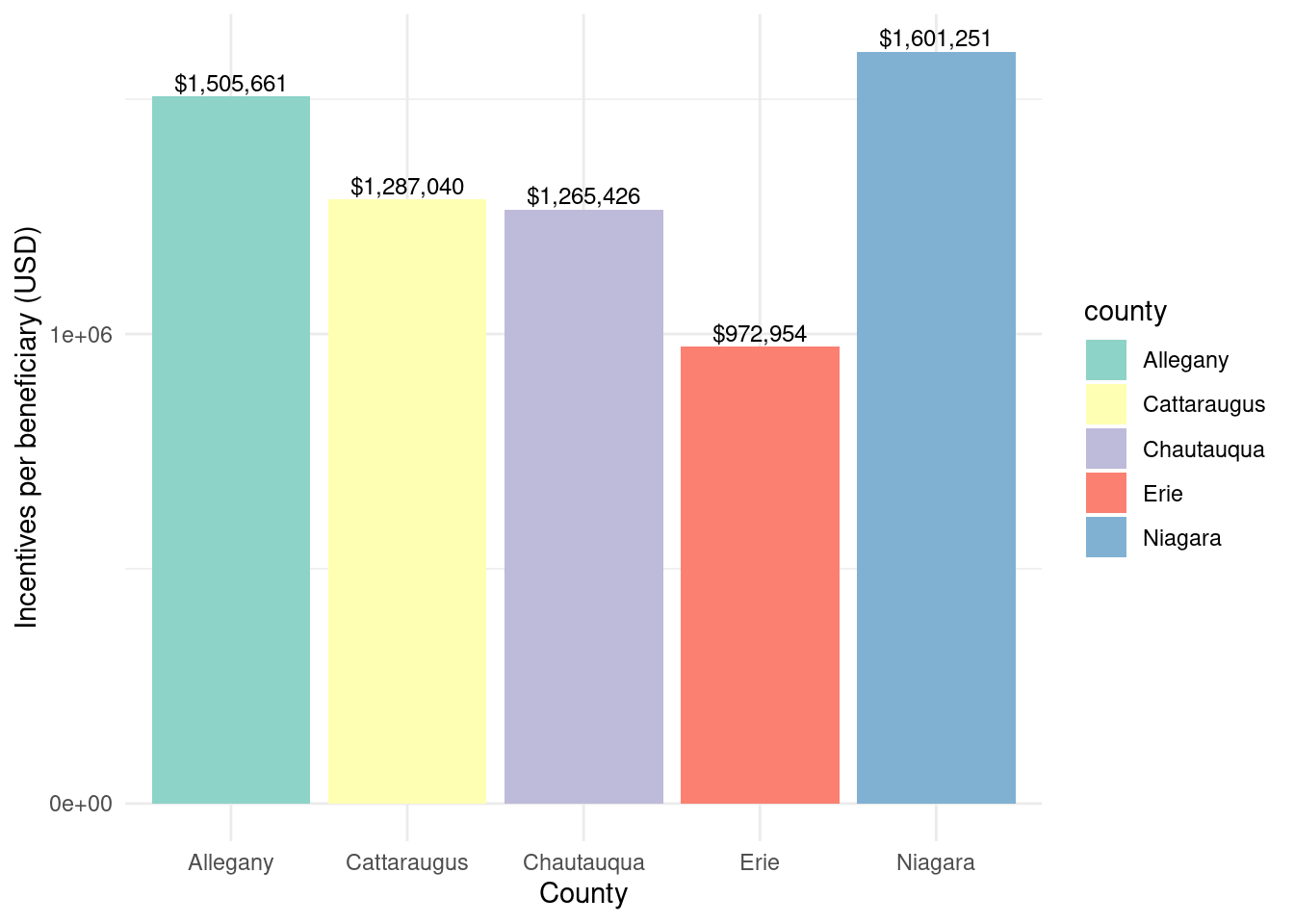
county_totalstats_nysun_largecomm_wny |>
  ggplot(aes(x = county, y = incentives_per_beneficiary, fill = county)) +
  geom_bar(stat = "identity") +
  theme_minimal() +
  labs(x = "County",
      y = "Incentives per beneficiary (USD)") +
  geom_text(aes(label = paste0("$", scales::comma(incentives_per_beneficiary, accuracy = 1))),
          vjust = -0.3,
          color = "black",
          position = position_dodge(width = 0.9),
          size = 3.2) +
  scale_fill_brewer(palette = "Set3") +
  scale_y_continuous(breaks = seq(0, 2000000, 1000000))

Total incentives per beneficiary by county for NY-Sun Large Commercial program

In [167]:

county_totalstats_nysun_largecomm_wny |>
  ggplot(aes(x = county, y = energycap_per_beneficiary, fill = county)) +
  geom_bar(stat = "identity") +
  theme_minimal() +
  labs(x = "County",
      y = "Energy capacity per beneficiary (kW)") +
  geom_text(aes(label = scales::comma(energycap_per_beneficiary, accuracy = 0.01)),
          vjust = -0.3,
          color = "black",
          position = position_dodge(width = 0.9),
          size = 3.2) +
  scale_fill_brewer(palette = "Set3")

Energy capacity per installed system by county for NY-Sun Large Commercial program